
|
|

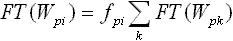
CisFinder is similar to RSAT oligo-analysis because it is based on clustering of over-represented short words (8bp) in the DNA sequence. However, we improved this method by clustering position frequency matrixes (PFMs) instead of exact words. PFM is estimated directly from counts of 8-bp words with and without gaps; then PFM is extended over gaps and flanking regions. Because these PFMs are long and carry additional information on nucleotide frequency, they are more reliable for clustering than exact words. CisFinder works >1000 fold faster than MEME and Weeder, and >100 fold faster than RSAT oligo-analysis. It can be used via web interface, but all components can also be downloaded and executed at the command line. The code is included (in C for computationally-intensive tasks, and PERL for utilities and web interface), so that you can compile the programs on any computer.
2. What can I do with CisFinder?
Here is a list of tasks you can do with CisFinder:
Other software for extracting genome sequences: RSAT or our PERL script extract_genome_seq.pl. We recommend using 200-bp sequences centered at the expected binding site of the TF. ChIP-chip usually has a lower spatial resolution, thus the size of sequences can be increased to 300 or even 400 bp. Upload your file using the "Upload New Data" menu (Fig.1)
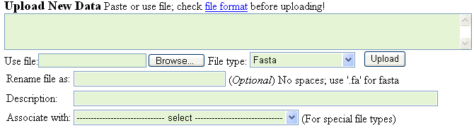
Fig. 1. Upload data menu
If you upload sequences generated with other software, the file type should be set to "Fasta", and the file name should end by ".fa" extension. You can also rename with ".fa" extension in the supplied field. We recommend adding a short description of the file for easier reference. After you have downloaded the fasta file, you can upload additional files associated with this fasta file: genome coordinates, evolutionary conservation, and attributes files (see file formats).
Select the uploaded file in the data file selection menu (Fig. 2) if it's not selected already. If you want to use a control sequence file, then select it in the 2nd line of the data file selection menu (Fig. 2). Control files help to reduce the number of false positives in results. Flanking sequences (e.g., 500-1000 bp away from binding sites) can be used as control; however this method may not work near CpG islands. If control file is not selected, then a 3rd-order Markov process is used to generate a random control sequence. After files are selected, click the "Identify motifs" button from the Analysis tools menu (Fig. 3).
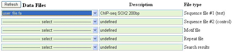
Fig. 2. Data file selection menu
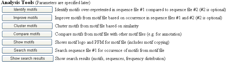
Fig. 3. Analysis tools menu
Parameters for motif identification will appear. "Select repeats for search" - use "No" as a default. The program assumes that repeats are lower-case characters in the fasta file. If the file is too short, it is worth to try including repeats into the search. Mammalian TF binding sites are often located in repeats (Bourque et al. 2008) thus searching repeats may be meaningful. False Discovery Rate (FDR) is used instead of p-values for multiple hypotheses testing; FDR = 0.05 is the recommended threshold. However if you want to see more motifs, you can increase it. The program generates at least 100 motifs (even if they are not significant). Option "Count motif once per sequence" is turned off as a default. If it is turned on, then control sequences are automatically truncated to the average size of test sequences because otherwise the comparison is meaningless. Search both strands of the sequence as a default. However, some sequences (e.g., near immediate promoters, splice sites, or 3'UTR of mRNA) need to be searched for one strand. Use the option "Adjust for CG/AT ratio and CpG" if you expect that control sequences are different from test sequences in their CG content; also try analysis without a control sequence in this case. Motifs can be ordered using different criteria, combining Z-score for over-representation (see Algorithms) with 3 optional criteria: (1) over-representation ratio ('ratio'), (2) information content (IC) ('info'), and (3) self-similarity ('repeat'), which contributes negatively to the score. IC and self-similarity may have both positive and negative effects on the quality of motifs. For example short fragments of transposable elements may have high IC, and they will be favored if IC is selected as a part of overall score. Motifs with high self-similarity generally have poor quality (e.g., repeats ATATATAT), but some of them are functional (e.g., CCCCNCCC for several zinc-finger TFs).
Maximum enrichment in repeats criterion is used only if the repeat file (see File format) is uploaded and selected in the 3rd line in the data file selection menu (Fig. 2). The default clustering method is by similarity measured by correlation between position weight matrixes (PWM) which are log-transformed PFMs (see Algorithms). Linkage (or co-occurrence) method is less sensitive than similarity, hence clusters may be smaller. However, it may work better for clustering motifs with high degree of self-similarity. Linkage method works better for longer sequences because of the increased number of motif pairs. If the option 'similarity and linkage' is selected, then linkage method is used only for motifs with a high level of self-similarity (average self-correlation of clustered PWMs > 0.5).
When results are generated, two buttons "Show elementary motifs" and "Show clusters of motifs"
can be used to visualize elementary motifs (before clustering) and clusters.
Clusters include an aligned set of member elementary motifs. Both files can be saved for
future reference: select which file to save, rename it if needed and edit the description.
Saved motif files can be edited: you can remove motifs of flip them (change to reverse
complementary motif). Also you can remove non-informative flanks of the motif and append
it to another motif file. Note that after clusters of motifs are saved, the information
on member elementary motifs may be lost.
5. Improving PFM with resampling
Motifs generated as described above generally have high-quality PFMs. However, matrixes
can be further fine-tuned using the resampling method. Resampling is an iterative
procedure; first PFM is used for search the sequence and select matching locations, and then
the PFM is updated based on nucleotide frequency distribution at selected locations.
Select the sequence (fasta) file in the 1st line of the data file selection menu (Fig. 2) if it's not selected
already. If you want to use a control sequence file (see above), then select it in the
2nd line of data file selection menu (Fig. 2). If a control file is not selected, a 3rd-order
Markov process is used to generate a random control sequence. Then select a motif file
which needs to be improved (3rd line of data file selection menu, Fig. 2). We recommend
you to use selected and preferably non-redundant motifs for resampling rather than raw
motifs identified by CisFinder (described above).
After files are selected, click the "Improve motifs" button from the Analysis
tools menu (Fig. 3).
Parameters for motif improvement will appear; most of them are the same as for
motif identification (see above). Three resampling methods are available:
(1) regression (default), (2) simple resampling, and (3) subtraction. Simple resampling
does not use the control sequence, whereas regression and subtraction use the control
sequence (see details in Algorithms). Select the number of iterations
and sub-iterations. The difference between them is that sub-iterations
using the same set of identified sites and only the rank of matching to motif is modified,
whereas iterations start with finding a new set of sites that match the motif.
Sub-iterations are much faster than real iterations and they can increase the speed
of the overall procedure.
6. Clustering DNA motifs
Motifs collected in any motif file can be clustered by similarity (correlation of
PWMs). Select motif file in the 3rd line of data file selection menu and click the
"Cluster motifs" button from the Analysis tools menu (Fig. 3). The only parameter
is similarity threshold.
7. Comparing DNA motifs with known motifs
Any two files with motifs can be compared with each other by similarity (correlation of
PWMs). Select the first motif file (e.g., results of motif identification)
in the 3rd line of data file selection menu (Fig. 2) and click the
"Compare motifs" button from the Analysis tools menu (Fig. 3). Then you can
select another motif file for comparison.
8. Searching sequence file for occurrence of motifs
Prediction of TF binding sites is based on finding locations in the sequence that match
the given binding motif represented by PFM or PWM. Select the sequence (fasta) file to be searched in
the 1st line of data file selection menu and a motif file with PFMs
in the 3rd line (Fig. 2). Then click the "Search motifs" button from the
Analysis tools menu (Fig. 3). There are two ways to control the stringency of
motif matching. The first method is to control the number of false positive matches
per 10 Kb of sequence length. The default is 5 false positive matches per 10 Kb of
random sequence. The second method is to select "Use existing thresholds" in the
"Number of false positives" pull-down menu. In this case, the program will use
pre-defined match thresholds that were either generated by the resampling module
(see details in Algorithms) or were uploaded together with the
motif file. Thresholds should be listed in the column called "Threshold"
(see File Formats), and a match is estimated as a sum of elements
of the PWM (log-transformed PFM, log10). If thresholds are pre-defined, then the
stringency can be modified by increasing/decreasing these thresholds by a certain
constant (pull-down menu "Add this value to the score threshold"). If an evolutionary
conservation file is uploaded for the sequence file, then conservation scores will
be listed for each predicted binding site in the output file.
The program removes overlapping and redundant motifs as follows. If two instances of the same motif overlap, then only one of them (with a higher match score) is retained. For example, palindromic motifs that match in both dirsctions are counted only once. In addition, if two different motifs overlap by more than 75% length, then only one is shown in the output. The option of removing overlapping and redundant motifs can be turned off; in this case all matches will be listed in the output.
Motif search results are immediately analyzed as described below, thus it is necessary to specify the interval for plotting the probability distribution of binding sites (100 bp is a default). Search results can be saved for future use.
9. Analyzing search results
Select the search results in the 5th line of data file selection menu (Fig. 2), then
click the "Show search results" button from the Analysis tools menu (Fig. 3). Two
tables are generated: a frequency table and an abundance table. The frequency table shows the
frequency distribution of binding sites along sequences aligned by their starting
position. For example, you can extract 2000-bp sequences from genome, centered at
binding sites identified by ChIP-seq, search for specific binding motifs and then
plot the distribution of motifs (Fig. 4). The peak in the middle (at 1000 bp) corresponds
to the binding site. In the case of POU5F1 presented in Fig. 4, there are several
binding motifs: OCT-SOX is the main motif, whereas OCT-3N-SOX (with 3-bp spacer)
is one of alternative motifs. It is seen that the OCT-3N-SOX peak is much lower than
the OCT-SOX peak and closer to background. The
frequency file contains raw data for Fig. 4: the abundance of motif in each strand,
and abundance of 50, 25, and 12.5% sites with the highest match score.
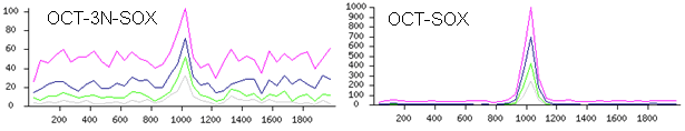
Fig. 4. Frequency distribution of composite motifs OCT-SOX and OCT-3N-SOX in 2-Kb
genomic regions centered at locations identified with ChIP-seq for transcription factor POU5F1
(data from Chen et al. 2008). Magenta line shows all sites matching to motifs
whereas blue, green, and gray lines show 50, 25, and 12.5% sites with the highest
match score.
The abundance table shows the number of motif matches in each sequence. It can be used
for classifying sequences based on the composition of binding motifs.
Click on the button "Show all motifs" to get a list of motifs with the total
count of matches for each motif. Click on the button "Show all sequences" to get
a list of sequences with the total count of matches for each sequence. If
genomic coordinates and/or attributes were uploaded in association with the
sequence file, then the table of sequences will include the coordinates and attributes
(e.g., closest genes). It is also possible to search sequences by name, number
of motif matches, or genes. If you click
on the sequence name, you will get a page with detailed information about the sequence and
motif matches. All motif matches are listed, and their coordinates are shown. If
coordinates were uploaded, then
hyperlinks will appear which lead to corresponding locations in genome browsers:
CisView (mouse genomes mm6 and mm9)
and UCSC genome browser
(other genomes). From this page, you can visualize the location of motifs by
selecting motifs (up to 3 motifs can be selected) and then clicking the button
"Show sequence". The sequence with highlighted binding motifs will appear.
10. Access to published data on DNA motifs, ChIP-chip, and ChIP-seq
One of the objectives for developing CisFinder was to provide a repository of public
data on ChIP-chip and ChIP-seq technologies in mammals.
11. File formats and uploading files
All files used in CisFinder are in plain text format and use tabs for delimiting
fields within one line. There is a total of 4 main types of files in the CisFinder: sequences, motifs,
search results, and repeats. Motifs can be submitted as PFMs and as degenerate
consensus sequences, which are converted to PFM form. These 4 types of files
may have 2 optional lines of annotation that start with the keyword "Parameters:"
and "Headers:." Parameters may specify the origin of the file, such as algorithm
parameters for derivation, whereas headers specify the columns of tab-delimited lines.
Aa additional 3 kinds of files can be associated with a sequence file:
genomic coordinates, attributes (e.g., gene names), and conservation scores.
11.1. Sequence files are in fasta format: the sequence name is preceded by ">" sign and the following lines contain the sequence. Maximum sequence length = 25Mb. Minimum recommended length = 5Kb; the program will process smaller files but has a low chance of finding a motif. Example:
>PET070528
AACCCAAAGTATGATATGCTATGATAGATAACCAAAAGGTAATATTATGAAATTTTTATCAACTATAATTATATAACTTG
AAACTGTTTCCTAAATCCGCCCTAGAGCTTACACAAAGCTGAGGGAAGTTTGCTGGAAAGTTCAGGCTGAGTGGGATGTT
>PET070400
TACTATTGGCGCTTCAATCAGTATTCGTCTTTTATAATACAATAATGCTATTTTGGATAAGTAAGTTTCTATTCAAGGAC
ACGTGTGGGCAGCTGTAACACTAATAATGTCCCATAAATAAGCGAGCAGAGCACATACTGCTGAGACAGACATGTAAGAA
............................................
To extract sequences from genome, make a tab-delimited text file with genome coordinates. The first line should indicate the genome (e.g., genome=mm10 or genome=hg38), other lines are either in bed format: (chr start end) or (name chr strand+/- length start). In the "Upload New Data" section of the menu select the file with coordinates. Alternatively you can paste the contents of the file into the top area. Select file type = genome location. Specify the name of the file to be generated in the "Rename file as:" field. This file will have fasta format, hence it's name should end with ".fa" extension. File description is optional. Sequence files can be modified in two ways by (1) extracting a subset of sequences, and by (2) extracting a specified region(s) from each sequence. To extract a subset of sequences go to the "Upload New Data" menu (Fig.1), open "File type" pull-down menu and select "Subset of sequences". In the "Associate with" pull-down menu, select the file from which sequences are going to be extracted, and paste a list of sequence names to be extracted (or specify file name with these sequence names). Specify a new file name with ".fa" ending in the "Rename file as:" box, add description, and push the "Upload" button. If the original sequence has associated files (coordinates, attributes, conservation) then this information will be transferred automatically to the new file.
To extract region(s) from each sequence, go to the "Data Management" menu (near bottom of the main page), select the sequence fasta file and push the "Sub-sequence" button. A dialog box will appear that asks for the name of the new file (don't forget the ".fa" ending!). The next dialog box will appear, where you need to enter the coordinates of the region to be extracted (positions are counted from zero). For example, "0-500" region corresponds to the first 500 bp of the sequence. Sub-sequences can be used for finding motifs over-represented in a specific region. For example, at the first step you have extracted 2000-bp long sequences centered at TF binding sites identified with ChIP-seq. To extract the central 200-bp regions of these sequences, specify the region: "900-1100". Motif frequency in this region can be compared to control flanking regions that are from 500 to 1000 bp away from binding sites. To extract flanking regions, use command "0-500,1500-2000". In this case, two regions will be extracted from each sequence (Fig. 8). If the original sequence has associated files (coordinates, attributes, conservation), then this information will be transferred automatically to the new file.
11.2. Motif files are formatted as follows. The first line starts with a ">" sign followed by motif name. The same line may contain additional tab-delimited fields:
| Pattern | (=consensus), |
| PatternRev | (=reverse consensus), |
| Threshold | (=threshold score), |
| Nmembers | (=number of member motifs in motif cluster), |
| Freq | (=number of motif matches in the test sequence), |
| Ratio | (=enrichment ratio of motif matches in the test sequence), |
| Info | (=information content of motif PFM), |
| Score | (=motif score used for ordering), |
| FDR | (=False Discovery Rate), |
| Repeat | (=enrichment ratio of this motif in repeat sequences), |
| Palindrome | (=1 if palindrome, and =0 otherwise), |
| Method | (=method of motif clustering: 0 for similarity, and 1 for co-occurrence), |
| Species | (=taxonomy of organism), |
| Parameters: | matchThresh=0.8500 | nucleotideOrder=A,C,G,T | |||||||||
| Headers: | Name | Pattern | PatternRev | Freq | Ratio | Info | Score | p | FDR | Palindrome | Nmembers |
| >SOX9 | CCWTTGTT | KAACAAWG | 12813 | 4.5857 | 9.407 | 176.0950 | 0.0000 | 0.0000 | 0 | 151 | |
| 0 | 2 | 72 | 13 | 13 | |||||||
| 1 | 3 | 72 | 2 | 23 | |||||||
| 2 | 46 | 1 | 2 | 51 | |||||||
| 3 | 1 | 2 | 1 | 96 | |||||||
| 4 | 1 | 1 | 1 | 96 | |||||||
| 5 | 2 | 4 | 93 | 1 | |||||||
| 6 | 3 | 2 | 2 | 93 | |||||||
| 7 | 6 | 26 | 13 | 55 | |||||||
| >OCT | HATGCWAA | ATTWGCAT | 404 | 3.1375 | 10.055 | 18.8350 | 0.0000 | 0.0000 | 0 | 4 | |
| 0 | 93 | 3 | 3 | 2 | |||||||
| 1 | 1 | 1 | 2 | 96 | |||||||
| 2 | 1 | 1 | 97 | 1 | |||||||
| 3 | 3 | 76 | 10 | 11 | |||||||
| 4 | 61 | 3 | 1 | 36 | |||||||
| 5 | 80 | 2 | 17 | 2 | |||||||
| 6 | 96 | 1 | 2 | 1 | |||||||
| 7 | 3 | 15 | 14 | 69 | |||||||
If motifs are uploaded as a pattern (consensus), then the file is formatted as follows:
| Parameters: | matchThresh=0.8500 | nucleotideOrder=A,C,G,T | ||
| Headers: | Name | Pattern | TFgroup | Info |
| >MIT_001NRF1 | RCGCANGCGY | NRF1 | 16 | |
| >MIT_002MYC | CACGTG | MYC | 12 | |
| >MIT_003ELK | SCGGAAGY | ELK | 14 | |
| >MIT_005NFY | GATTGGY | NFY | 13 | |
| >MIT_006SP1 | GGGCGGR | SP1 | 13 | |
| >MIT_007AP1 | TGANTCA | AP1 | 12 | |
| >MIT_009ATF | TGAYRTCA | ATF | 14 | |
| >MIT_010YY1 | GCCATNTTG | YY1 | 16 |
11.3. Search results are formatted as a tab-delimited text file with the following columns: MotifName, SeqName (sequence name), Strand, Len (motif length), Start (starting position counted from 0), Score (matching score), Sequence (matching sequence), and Conservation (evolutionary conservation score, from 0 to 100). The "Parameters:" line should specify the name of the sequence (file_fasta) file that was searched and the motif name that contain PFM (file_motif). Here is an example of search results:
Parameters:	file_motif=public-motif_pluripotent	file_fasta=public-P300_binding.fa
Headers:	MotifName	SeqName	Strand	Len	Start	Score	Sequence	Conservation
STAT3	Chen2008P300000002-900-1100	-	9	119	4.3932	TTCCCGGAA	40
TEF	Chen2008P300000005-900-1100	-	8	87	3.3398	AGGAATGC	0
NANOG	Chen2008P300000004-900-1100	+	9	116	3.5202	CCACTTCCT	1
KLF	Chen2008P300000004-900-1100	+	8	96	3.7154	CTCCACCC	1
KLF4	Chen2008P300000004-900-1100	+	9	109	4.0565	GCCACACCC	1
SOX9	Chen2008P300000003-900-1100	-	8	60	3.7513	CCATTGTT	28
11.4. Repeat files are formatted as a list of repeat motifs, each described with 2 lines. The first line has 5 tab-delimited fields:
11.5. Genome coordinates files have the following 5 columns (tab-delimited): Sequence Name, chromosome, strand, blockSize, startingPosition. The first line shows the genome, e.g. mouse mm9 or human hg19.
Here is an example of coordinates file:
Parameters:	genome=mm9
Chen2008Nanog000001	chr1	+	2000	10016005
Chen2008Nanog000002	chr1	+	2000	100755619
Chen2008Nanog000003	chr1	+	2000	101316192
Chen2008Nanog000004	chr1	+	2000	102617082
Chen2008Nanog000005	chr1	+	2000	102707398
To upload a file with coordinates, select "Genome location" in the "File type" pull-down menu (Fig. 1); select the sequence (fasta) file with which genome coordinates are associated (both should have matching sequence names) in the "Associate with" pull-down menu. Do not fill in the "Rename file as" box because the coordinate file will be automatically renamed as the name of sequence file plus a ".coord" ending. Do not fill in a description either.
11.6. Sequence attributes files have multiple columns (tab-delimited). The first column has sequence names. Column names are listed in the "Headers" line (which is a starting line). Use the header "Symbols" for gene symbols, and "Distances" for distance to gene transcription start site (TSS). Several gene symbols can be separated by commas; in this case, distances are also comma-separated. Distances are negative if a sequence is located upstream of TSS and positive if it is downstream of TSS. Here is an example of attribute file:
Headers:	Name	Symbols	Distances
Chen2008P300000001	Sulf1	156
Chen2008P300000006	Tmem131	-46164
Chen2008P300000010	Pecr,Tmem169	22150,-22285
Chen2008P300000015	Armc9,Htr2b	33225,-76052
To upload a file with attributes, select "Sequence attributes" in the "File type" pull-down menu (Fig. 1); select the sequence (fasta) file with which genome attributes file is associated (both should have matching sequence names) in the "Associate with" pull-down menu. Do not fill the "Rename file as" box because the attribute file will be automatically renamed as the name of sequence file plus ".attr" ending. Do not fill in a description either.
11.7. Sequence conservation files have a fasta format; the sequence name is preceded by a ">" sign and the following lines contain conservation scores for the sequence, comma separated. Conservation scores range from 0 to 100 and can be downloaded from UCSC web site (there it ranges from 0 to 1, hence it needs to be multiplied by 100). The first line in the file should specify parameters: interval and genome. Normally we use interval=5, which means that each conservation score correspond to 5 bp of the sequence. If an interval is not described it is assumed to =1. If the genome is not specified, then sequences cannot be visualized in genome browsers. Here is an example of conservation file:
Parameters:	interval=5	genome=mm9
>Chen2008P300000006
2,2,2,4,7,8,11,12,11,7,8,7,5,4,3,2,2,3,3,2,1,0,1,1,1,3,3,0,0,0,0,0,0,0,0,0,1,1,0,0,0,0,0,1,0,0,0,1,0,1,
3,1,1,3,4,2,3,4,4,3,0,1,0,1,1,0,0,10,27,36,47,72,64,48,27,1,2,16,22,25,35,40,11,4,4,3,4,5,6,0,0,5,10,11,4,1,0,3,0,2,
42,55,20,0,0,0,0,2,1,0,0,0,0,0,2,0,0,0,0,0,0,0,0,0,0,0,0,0,0,1,2,0,0,0,1,1,0,0,1,1,0,0,0,1,1,0,0,0,0,0,
0,2,2,0,0,7,21,24,17,5,2,1,1,3,5,7,4,0,0,0,1,3,4,4,3,11,12,12,9,4,1,0,1,0,0,0,0,1,2,2,1,2,1,0,0,0,0,1,0,2,
5,8,10,3,0,1,1,2,0,0,0,4,0,0,0,0,1,3,6,3,1,0,0,0,0,0,1,2,4,6,5,2,2,4,4,13,26,45,57,63,66,66,62,55,41,19,10,5,3,2,
2,5,8,7,4,0,0,0,0,0,0,0,0,2,4,4,4,3,3,1,1,0,1,4,3,1,2,6,7,5,3,7,13,20,28,32,34,39,40,38,32,19,9,1,0,1,2,1,1,0,
1,4,2,0,0,6,6,2,1,0,0,0,0,0,1,2,3,0,0,1,4,4,2,1,0,0,0,1,2,0,1,0,0,0,0,0,1,0,1,1,1,1,0,1,12,20,25,26,23,15,
11,11,21,28,30,28,23,24,27,30,33,35,38,40,39,38,38,34,25,15,9,6,4,4,3,4,8,8,9,12,14,12,6,2,1,0,0,0,0,1,3,3,4,9,12,13,14,9,3,1,
>Chen2008P300000007
0,0,1,3,4,4,3,2,1,1,2,2,3,5,4,1,1,0,0,0,0,0,0,0,0,0,0,0,0,0,0,0,0,0,0,0,0,0,0,0,0,0,0,0,0,0,0,0,0,0,
0,0,0,0,0,0,0,0,0,0,0,0,0,0,0,0,0,0,0,0,0,0,0,0,0,0,0,0,0,0,0,0,0,0,0,0,0,0,0,0,0,0,0,0,0,0,0,0,0,0,
0,0,0,0,0,0,0,0,0,0,0,0,0,0,0,0,0,0,0,0,0,0,1,1,1,1,1,0,0,0,0,0,2,12,23,28,30,34,37,35,29,22,16,15,17,16,10,6,3,2,
4,6,7,8,8,8,6,4,2,4,5,4,1,1,2,2,3,5,6,4,1,2,1,1,2,2,2,1,1,3,6,7,8,10,12,10,8,11,18,22,21,17,11,9,9,7,2,1,0,1,
0,0,0,1,3,3,0,1,18,21,14,0,0,0,0,0,0,0,0,0,1,9,6,0,0,0,0,0,0,0,0,0,0,0,0,0,0,0,0,0,0,0,0,3,1,0,0,0,0,0,
0,0,0,0,0,0,0,0,16,58,97,57,1,11,40,39,87,92,41,24,2,30,28,1,15,99,92,96,97,99,100,100,98,100,95,100,100,100,100,84,87,100,100,100,100,100,100,100,100,100,
100,100,100,100,100,100,100,100,100,99,98,99,100,97,99,100,100,99,99,100,100,98,100,78,88,100,100,100,100,100,99,77,16,49,99,98,99,100,100,99,93,19,2,0,4,5,12,46,100,100,
100,100,100,44,2,3,15,96,100,100,100,87,92,98,99,99,33,0,3,17,61,81,88,95,100,100,100,100,98,100,100,100,99,21,81,89,98,100,100,100,99,100,99,98,100,100,100,100,99,100,
To upload a file with conservation, select "Conservation" in the "File type" pull-down menu (Fig. 1); select the sequence (fasta) file with which the conservation file is associated (both should have matching sequence names) in the "Associate with" pull-down menu. Do not fill the "Rename file as" box because the attribute file will be automatically renamed as the name of sequence file plus ".cons" ending. Do not fill in a description either.
12. Algorithms
12.1. Estimating position frequency matrix (PFM) from 8-mer word counts
The proposed algorithm is based on estimating PFM directly from 8-mer word counts in the
test and control sequences. We will start with a numerical example to make the algorithm
clear, and then will proceed to the formal justification of the method.
Consider a specific 8-mer word W (e.g., W = "ATGCAAAT") which has T(W) = 200 matches
(instances) in the set of test sequences and C(W) = 50 matches in the set of control
sequences. For simplicity, we will not consider the distribution of word instances in
individual sequences within the test set and control set and will count only the total
number of instances as if all sequences in a set are concatenated. However, the CisFinder
has an option to count only one match of each word per sequence. The total length of all
test sequences and all control sequences is assumed to be the same (3 Mb, in this example).
For word W, we define a nucleotide substitution matrix [Wpi] which contains words that are
derived from W by placing a nucleotide i in position p:
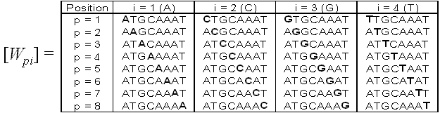
Fig. 5. Nucleotide substitution matrix derived from word W = "ATGCAAAT".
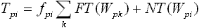
The frequency of each word from the nucleotide substitution matrix counted in the same target sequence makes the frequency substitution matrix (Fig. 1B). For convenience, we will use brief notations Tpi = T(Wpi) and Cpi = C(Wpi) for the frequency of word Wpi matches in the test and control sequence sets (elements of frequency substitution matrixes):
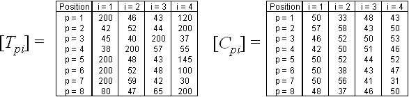
Fig. 6. Frequency substitution matrixes for the test and control sequence sets.
The proposed method to estimate PFMs is
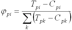 | (e1) |
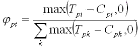 | (e2) |
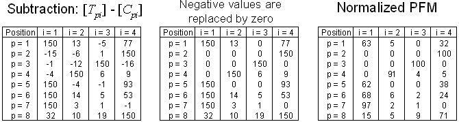
Fig. 7. Estimation of PFM in 3 steps: subtraction of frequency substitution matrixes,
replacing negative values by zeroes, and normalization.
This method is justified from the following model. Let us assume that a TF binds to a set of locations in the genome where corresponding DNA sequences can be aligned together. Using this alignment, we can estimate the frequency, fpi, of each nucleotide i in each position of aligned sequences, p, which is the element of the PFM. We further assume that binding strength of the TF is additive with no interaction between positions. This simplification is justified by the fact that all existing databases use PFMs to describe TF motifs, and this strategy works reasonably well. A successful ChIP-seq experiment generates a set of genome locations which is enriched in TF binding sites. The test set of sequences typically consists of 200-bp long segments centered at projected binding sites, whereas the control set of sequences can be taken away from binding locations (e.g., 500 bp away). In example shown in Fig. 8, there are 2 control sequence fragments near each projected binding site. It does not matter that control sequences are longer than test sequences because the frequency of words in the control set of sequences, Cpi, is automatically adjusted to sequence length. However, if word frequencies are counted only once per individual sequence, then sequence length should be the same in the test and control data sets.
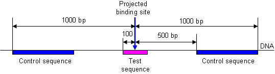
Fig. 8. Example of selecting test and control sequences.
Consider a word W with a sequence of nucleotides that corresponds to the maximum values of the PFM at each position. This word is then used to generate frequency substitution matrixes [Tpi] and [Cpi] for the test and control sets of sequences, respectively. Each instance of word Wpi in the test or control sequences can either correspond to a true binding site of the TF (we call it functional) or not (non-functional). Factors determining functionality of different instances of the same DNA word are largely unknown and may include sequence context and chromatin status. Because the probability of TF binding is proportional to PFM elements at each position (assumption of additive contribution of each position to TF binding), the number of functional instances, FT(Wpi), of word Wpi in the test sequences is proportional to fpi:
 | (e3) |
 | (e4) |
 | (e5) |
Because the PFM is estimated as a difference between word counts in the test and control sets of sequences (e1,e2); thus, the variance of PFM elements is equal to the sum of variances of word counts in the test and control sequences. The variance of word counts is very close to the mean, which is expected from the Poisson distribution (we checked it using pseudo-random sequences generated with the 3rd order Markov process). For example, if word counts are 120 in the test set of sequences and 40 in the control set (i.e., 3-fold over-representation), then the relative error (accuracy) is equal to sqrt(120+40)/(120-40) = 0.158.
12.2. Implementation of the method for PFM estimation
A successful ChIP-seq experiment generates a set of genome locations that are enriched in TF
binding sites. For a test sequence set, we usually extract 200 bp sequence segments centered
at a peak of projected TF binding sites. For a control sequence set, we usually extract
500 bp sequence segments starting from nucleotide positions 400 bp away from both ends of
200 bp test sequence segments. (However, the CisFinder allows users to choose different
sequence lengths). The CisFinder identifies binding motifs of TFs using direct counts
of all possible 8-mer words with and without gaps in both test and control sequence sets
(Fig. 9). This word length was selected experimentally based on the observation that
longer words have too few matches in target sequences, whereas shorter words may fail to
capture the most informative portion of the motif and show lower rates of over-representation.
(Note: the command-line version of CisFinder allows the use of 6- and 10-mer words).
Word counts are stored in the array of integers. Although there are many different ways
to insert gaps in the 8-mer words, we consider only 8 specific patterns of gap insertions
(Fig. 9). We found that this limited set of gap insertion effectively helps to capture
composite motifs with multiple functional elements. For example, search for a word
"ATGCAAAT" with a 2 bp gap in the middle is equivalent to the search for word "ATGCNNAAAT".
PFM is then estimated for each word based on >1.5 fold (default threshold) enrichment in
the test sequences compared to the control sequences using (e2). The fold enrichment
criterion is optional (it can be set to 1).
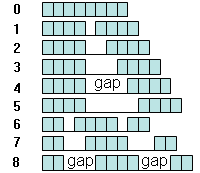
Fig. 9. Words with and without gaps used for searching of over-represented motifs.
Over-representation of word counts in the test sequences, T, compared to the control sequences, C, is then evaluated using a z-score which is estimated based on the hypergeometric probability distribution. Let us first consider the case where only one instance of each word is counted per each sequence of equal (or approximately equal) length. The proportion of sequences, q, with a given word in the set of test sequences is compared with the proportion of sequences, p, with the same word in the combined set of test and control sequences (if the null-hypothesis is true then test and control sets of sequences can be combined) with z-score:
| z = (q - p)/sqrt[p*(1-p)*(N-n)/(N-1)/n], |
where n is the number of test sequences, and N is the number of combined test and control sequences. If multiple instances of each word are counted per each sequence, then the method is modified as follows. The set of test sequences with the total length T is split into T/m segments of length m, where m is the actual length of the word including gaps. Each instance of the word is then associated with the segment where it starts. Because overlapping instances of the same word are counted as one instance, there are not more than one instance associated with the same segment. Similarly, the set of control sequences with the total length C is split into C/m segments of length m. We use the same equation for the z-score (see above) where q is the proportion of test segments with the word, p is the proportion of test and control segments with the word, n = T/m, and N = (T + C)/m. Although occurrences of word instances in adjacent segments may be weakly correlated, the hypergeometric distribution gives a reasonable approximation of the z-score. To fill the gaps and extend the length of PFMs, the test and control sequences are searched again for the exact match to each word with z > 1.643 (to satisfy the condition of p < 0.05 for one-tail z-test). Each match of the word in the test (or control) sequence is then examined for nucleotides in the gaps and flanking sequences (2 bp at each side) that are not included in the word. In this way, we can count nucleotide frequencies in gaps and flanking regions and estimate the PFM for these positions using (e2) (Fig. 10). The program is also designed to trim flanking sequences if they are not informative (if the ratio of maximum frequency to minimum frequency is <3). To increase the information content of PFMs, we use the contrasting procedure: the median of minimum PFM values at each position is subtracted from all PFM values; negative values are then replaced by zero; and the PFM is re-normalized.
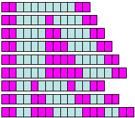
Fig. 10. Extending the position frequency matrix (PFM) over
flanks and gaps with equation (e2)
The frequency distribution of nucleotides in the flanking regions and in gaps of a certain word may differ substantially between the test and control sets of sequences, and this difference can be used to increase the statistical power for identification of significant motifs. Frequency distributions of nucleotides (counted for each nucleotide and each flanking/gap position) in the test and control sequences were compared using the G-test (Sokal and Rohlf 2001). Assuming that this test is independent from the z-test for over-representation of word counts (see above), we combined p-values from these tests using Fisher's method (Hess and Iyer, 2007. BMC Genomics, 8:96). Then, False Discovery Rate (FDR) is estimated using method of Benjamini and Hochberg (1995) to account for simultaneous testing of multiple hypotheses. The program generates at least 100 top-score motifs, and additional motifs are limited to those that satisfy the criterion of FDR < 0.05. Flanking positions are trimmed if the ratio of maximum frequency to minimum frequency is <3.
12.3. Clustering of motifs
Motifs are clustered based on similarity and/or co-occurrence (Fig. 9). Various methods
were proposed to measure the similarity of PFMs including Bayesian models. Here we use
a simpler method and measure similarity by Pearson correlation between elements of the
corresponding position-weight matrixes (PWMs) for all overlapping positions, where PWM is
derived from PFM by log-transformation: : xij = log(pij/qj),
xij is the weight of nucleotide j in position i, pij is the probability to
find nucleotide j in position i, and qj is the background frequency of
nucleotide j. For simplicity, here we assume equal background
frequencies (qj = 0.25); zero probabilities are avoided by adding pseudocount =1
to nucleotide counts in the PFM. Offset and orientation of motifs is selected based
on maximum correlation, restricted to the minimum overlap of 6 bp and maximum
overhang of 2 bp. Because correlation is estimated for a minimum of 6 overlapping
positions, there are at least 24 points (6 positions x 4 nucleotides) for estimating
correlation. Thus, even low correlation is significant (e.g., r=0.5; d.f.=22; p<0.05).
The default correlation threshold in CisFinder (r=0.7) is always significant, however the
user can adjust the correlation threshold to increase or decrease the size of clusters.
We use single-linkage clustering, and then each cluster is checked for homogeneity. If the
cluster is not homogeneous, it is separated into sub-clusters using the second round of
clustering. Sub-clustering is done iteratively starting from a pair of seed motifs by
sequential addition of most similar motifs and re-estimating the combined PFM for the
sub-cluster. Each pair of motifs is characterized by the score = r*m1*m2, where r is
the correlation between PWMs, and m1 and m2 are the number of linked members for motif
1 and motif 2, respectively. Then the pair with the highest score is selected as a seed
for the sub-cluster. This procedure is different from the original single-linkage
clustering because motifs are added to the sub-cluster based on the similarity to
the combined PFM of all motifs that are already included into the subcluster, whereas
original clustering is based on the similarity between individual (non-combined) motifs.
Motifs are added until no motif within the cluster can be added to the
sub-cluster using the given threshold of similarity. If all elements in the cluster
appear to be in the same sub-cluster, then the cluster is considered homogeneous.
Otherwise, the elements of the sub-cluster are removed from the cluster, and the same
algorithm is applied to the remaining elements.
The advantage of clustering PFMs compared to clustering words (as in RSAT) is that PFMs contain more information than words alone. Words differ qualitatively (the nucleotide either matches or mismatches) whereas PFMs differ quantitatively (i.e., the probability of each nucleotide correlates between two PFMs). Motifs within the same cluster are then arranged using the hierarchical clustering with cluster flips to place similar motifs near each other (Eisen et al. 1998). Then, the PFM for the entire cluster is estimated as the weighted average of member PFMs using local information content at each position p (estimated for the position p and its two neighboring positions at both sides) multiplied by motif abundance as a weight. Finally, a sequence logo (Schneider and Stephens 1990) is generated from the PFM (Fig. 12).
Co-occurrence of word instances in the test sequence is used as an alternative criterion for clustering. This method is generally less accurate because of the limited number of word pairs in the sequence. However, it works better for clustering PFMs with high level of self-similarity (after position shift by 1-4 bp), because their relative position cannot be uniquely identified based on correlation. The use of co-occurrence clustering method is optional and can be used either globally or only for PFMs with high level of self-similarity.
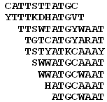
Fig. 11.Clustering of motifs based on similarity of PFMs and/or co-occurrence

Fig. 12.Sequence logo generated from combined PFM
12.4. Search for motifs that match to a PFM
Finding DNA sites that match a specific PFM in a given sequence is computationally intensive
if a matching score is estimated sequentially at each position of the sequence as in
MatInspector or MATCH. We propose a faster method to identify DNA sites, which
is based on a lookup table. For each motif represented by a PFM, we selected the most
informative stretch of 8 nucleotides, which is used as a core. Then a lookup table
is generated which specifies all PFMs from the list, whose cores match sufficiently
well to each possible 8-mer word. The length of 8 bp for the core is selected because
the number of all 8-mers is small enough to keep the lookup table in the computer memory,
and 8-mer words are enough specific to be linked with only a few PFMs that match them.
A match score is defined as a log likelihood that a specific sequence matches a matrix;
it is equal to the sum of those elements of the PWM (log-transformed PFM) which
correspond to nucleotides at each position of the sequence. The match score for the
full matrix, Tfull = T8 + Tresid, where T8
is the match score for 8-mer core and Tresid
is the match score for the residual of the matrix. The program finds the threshold
value R8 for the match score T8, which ensures that the match
score for the full matrix
exceeds the given threshold Rfull with probability 0.999 if T8 > R8:
| R8 = Rfull - F-1(0.999) | (e6) |
12.5. Resampling algorithms
Three algorithms are available for resampling: simple resampling, regression, and
difference-based. In all algorithms, the motif matching score is estimated as a sum of
elements of the PWM that correspond to the sequence at each position. Match threshold
is adjusted according to the expected number of false positives per 10,000 bp in
control sequence.
Simple resampling: in each iteration, find matching motifs with score ≥s and
then set the PFM equal to the frequency of nucleotides in matching motifs.
Regression: in each iteration, find matching motifs with score ≥s and
estimate the frequency of nucleotides in matching motifs in the test and control
sequences. Do linear regression of log-transformed nucleotide frequencies in the test
sequence versus corresponding log-transformed nucleotide frequencies in the control
sequence. Then the PFM is adjusted to bring individual points closer to the
regression line. The idea behind the method is to equalize the stringency of matches
between motif positions and individual nucleotides.
Difference-based: in each iteration, find matching motifs with score ≥s and
estimate the frequency of nucleotides in matching motifs in the test and control
sequences, then set the PFM equal to the difference between nucleotide frequency
in the test file and nucleotide frequency in the control file (replace negatives
with zero).
13. Enable scripted windows in the browser
CisFinder often opens new windows for data processing rather than continue
in the same window. Thus, you will need to enable pop-up windows to
use it successfully.
Other programs (such as Google toolbar) may also
prevent pop-ups. To disable them, refer to the
Disable Pop-Up Blocking for WebCT section on the WebCT Tuneup page.
14. Terminology and feedback
False Discovery Rate (FDR)
Feedback
Contact Alexei Sharov sharov (at) comcast.net
if you have problems with CisFinder or suggestions for improvement.