| Home | Analysis | Services | Resources | Contact | About |
|---|

Analysis of gene expression dataMain advantages of ExAtlas software for gene expression statistical analysis are the following:
The workflow in ExAtlas is shown below. Detailed descriptions and step-by-step instructions are available in the in the exatlas-help file. Two main types of data files are gene expression profiles and gene sets, which can be uploaded manually or retrieved from GEO database. Tools for comparison of two or more data sets are shown as yellow boxes.
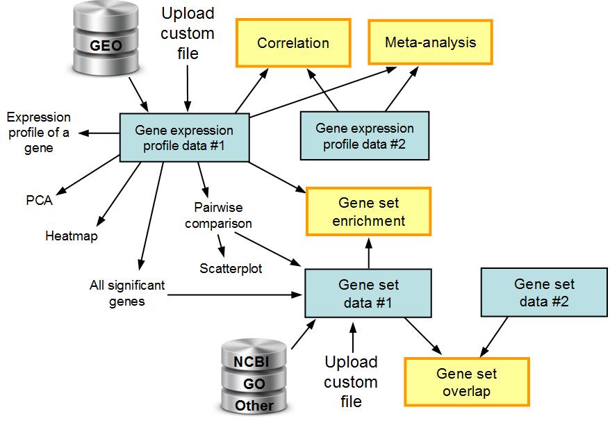 Fig. 1. The workflow in ExAtlas. Gene expression data can be uploaded manually as tab-delimited text files, which are normalized as transcripts per million (TPM) during the upload. Preloaded public data sets improve the functionality of the software because they save time on data search, retrieval, and preprocessing. Users can store their data files indefinitely in their account and keep using them for additional analyses. The file management system allows users to download, delete, or edit their data files. ANOVA is used in ExAtlas to evaluate the variability of log-transformed gene expression values between replications. First, one-way ANOVA is applied to each individual gene (or probe in the array), and then the error variance (also known as mean square error) is adjusted to the results obtained for other genes. Error variance may appear very low by pure chance for some genes, especially if the number of replications is small; and this factor may increase the number of false positives. Error models used in ExAtlas are designed to get a better estimate for the true error variance than the error variance estimated from expression of a single gene (i.e., empirical error variance). Adjustment is done by taking the maximum of the empirical error variance for a single gene and the average error variance for multiple genes that are expressed at approximately the same level as the given gene. The average errov variance is estimated as follows. All genes are sorted based on the average log-expression in all samples, and then the average error variance is estimated in a sliding window of 500 genes. The top 1% of genes with highest empirical error variances are not counted in this calculation to avoid potential bias due to outliers and highly variable genes. Low-expressed genes generally have higher error variances than high-expressed genes. However, their variation could be underestimated due to data processing (e.g., using cutoff thresholds, rounding, or pseudo-values). Thus in ExAtlas, the average error variance is forced to increase monotonically with decreasing expression of genes below the median. According to the default error model, adjusted error variance equals the maximum of the empirical error variance and the average error variance. Other error models are available when users select the option "Run ANOVA again." These include using empirical error variance without adjustment, or average error variance, or Bayesian correction of error variance, or the maximum between empirical error variance and its Bayesian correction. With ExAtlas, users can run ANOVA-like analysis even for data sets with no replications (this option is usually not available in other software). In this case, the error variance is estimated based on the half-normal probability plot method. We assume that at least a half of degrees of freedom in a set of gene expression values represent random effects. Thus, the standard deviation, σ, of random effects can be approximated by the median of positive deviation (i.e., absolute value of deviation) from the mean divided by 0.675 (inverse half-normal cumulative distribution for p=0.5). The error variance in ANOVA is then set to σ2. This method is applied to each set of the 500 genes in a sliding window that is shifted across the set of all genes sorted by their average log-expression. This error variance is then used for evaluating the significance of gene expression change in individual genes. Specificity of gene expression in a specific tissue or cell type is evaluated by a z-value that compares expression in a given tissue with the average expression in other tissues that are not correlated with the tested tissue. Tissues are considered correlated if the log-transformed multidimensional distance of their log-transformed expression profiles is less than 1/3 of the maximum distance between tissues measured by PCA. Specificity of a gene is considered significant if z > 2. Heatmap and PCA are used to explore gene expression profiles of all tissues or cell types in a data set. These methods can be applied to a subset of genes that satify criteria of significance (thresholds of FDR and fold change). By default, both the heatmap and PCA are applied to averages of log-transformed gene expression in each tissue, but there is an option to use individual replications for analysis. PCA determines major correlations among gene expression profiles in a data set. Users can check the box "PC gene clustering" to identify genes that are correlated positively and negatively with each principal component. In the heatmap, both columns and rows are sorted by hierarchical clustering. However, if the number of genes is >2000, then rows (genes) are clustered by PCA: first by positive and negative values of each PC that exceed 1/4 of the maximum value, then by combinations of values in each pair PCs (both >1/4 of the maximum value and the ratio between PCs < threefold). Residual genes that matched neither to individual PCs nor to their pairs are placed at the end of the heatmap and sorted by PC1. Correlation between gene expression profiles can be identified in ExAtlas in order to detect functional similarity between cell types or tissues. Thus, it helps in functional annotation of transcriptome changes. For example, the function of various transcription factors (TFs) can be inferred from the expression change of downstream genes after induction (or repression) of these TFs in cultured pluripotent cells (embryonic stem cells ESC or induced pluripotent stem cells iPSC). Such experiments has been done with several humdreds of mouse and human TFs, and the results are included as public resources in ExAtlas. Genes that do not show significant change of expression may add noise to correlation analyses. Thus, it is reasonable to analyze only those genes with significant change of expression in both data sets. If the correlation between gene expression profiles is positive and significant, then we expect that the number of genes upregulated in both profiles or downregulated in both profiles (called "coregulated" genes) is larger than expected in pairs of noncorrelated gene expression profiles. To identify coregulated genes and evaluate their statistical significance, users select option "Identify coregulated genes" before doing correlation analysis. Statistical significance is evaluated by EPFP, which is similar to FDR but is not estimated from p-values. The algorithm for finding coregulated genes is based on the analysis of data points in the positive quadrant (i.e., x > 0 and y > 0) for upregulated genes, and negative quadrant (i.e., x < 0 and y < 0) for downregulated genes, where x and y are expression values of a gene (i.e., log ratio vs. median or other baseline) in samples compared from data sets #1 and #2, respectively. Because the analysis of upregulated and downregulated genes is identical except for the direction of expression change, the algorithm is described here only for the upregulated genes. First, gene expression change values are replaced by their rank order in the positive quadrant. If the null hypothesis holds (i.e., no correlation), then genes are expected to have a uniform random distribution (Fig. 2B). However, if gene expression profiles are positively correlated, then more genes (points) can be found near the upper right corner of the plot (Fig. 2B). To estimate EPFP(rx,ry) for a gene with rank orders rx and ry in the first and second expression profile, respectively, the density of dots/genes is estimated in a dark-shaded rectangle in Fig. 2B, and compared to the density of dots in two adjacent light-shaded rectangles. The EPFP equals the density of dots in the light-shaded area divided by the density of dots in the dark-shaded area. Because we have two light-shaded rectangles, EPFP is estimated twice, and then the largest value is selected (to be conservative). Because EPFP may not monotonically decrease with the increasing rank of genes, it is forced to decrease monotonically. In particular, if EPFP(rx1,ry1) > EPFP(rx,ry), rx1 > rx, and ry1 > ry, then EPFP(rx1,ry1) is reassigned to EPFP(rx,ry). All genes with EPFP below a selected threshold are considered coregulated (Fig. 2C). To identify oppositely coregulated genes (i.e., upregulated genes in file #1 that are downregulated in file #2), the direction of change in file 2 is set to "Reversed." The gene expression change in file 2 is thus inverted (i.e., multiplied by -1), and oppositely coregulated genes can be identified in the same way as shown in Fig. 2.
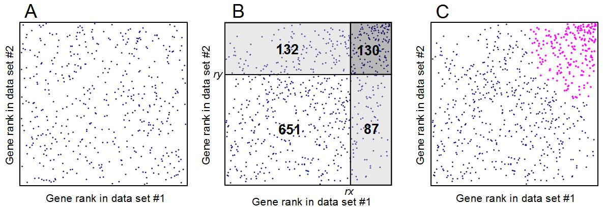 Fig. 2. Estimating the expected proportion of false positives (EPFP) for positively coregulated genes: (A) scatterplot of gene expression ranks in the positive quadrant if there is no correlation. (B) The same plot if gene expression profiles are correlated; numbers indicate gene counts in each area. The density of dots/genes in the dark-shaded rectangle is compared to the density of dots in two light-shaded rectangles used as baseline, generating two estimates of EPFP for a gene at the lower left corner of the dark-shaded rectangle (with expression rank orders rx = 651 + 132 = 783 and ry = 651 + 87 = 738): EPFP1 = 0.281 and EPFP2 = 0.237. The greater value of these is then selected: EPFP = 0.281. (C) All coregulated genes with EPFP ≤ 0.3 are highlighted in magenta.
Gene set overlap and gene set enrichment analyses are used to evaluate if specific gene sets (such as GO or KEGG) are overrepresented among upregulated and/or downregulated genes. For example, if a set of upregulated genes, S1, is identified using threshold values of FDR and/or fold change, then we can test if this set is enriched in genes that belong to a set of annotated genes, S2. The proportion of genes from set S2 in the genome genes equals p = n2/N, where n2 and N are the numbers of genes in S2 and in the whole genome, respectively. The proportion of genes from set S2 within set S1 is equal q = m/n1, where m is the number of common genes in S1 and S2, and n1 is the number of genes in S1. Genes that are common in sets S1 and S2 belong to the overlap of these two sets (i.e., S1⋂S2); thus, the goal of the analysis is to check if the overlap can (or cannot) be explained by a random draw of genes. In particular, we can say that genes from set S2 are enriched in the set S1 if the overlap of genes in sets S1 and S2 is greater than can be explained by random choice. Z-values are then estimateed assuming that the proportion of common genes has a hypergeometric probability distribution. Gene set enrichment analysis is similar to the method of gene set overlap, but it has a greater statistical power because it does not require defining thresholds for delineating sets of differentially expressed genes. In particular, gene set enrichment analysis can find significant associations with functional gene sets even if there are no significantly upregulated genes based on standard criteria (e.g., FDR ≤ 0.05 and fold change ≥ 2). Gene set enrichment analysis uses the order of genes sorted by the change of their expression to identify the best threshold to delineate the set of differentially expressed genes. Among various approaches to gene set enrichment analysis, we selected Parametric Analysis of Gene Enrichment (PAGE) because of its simplicity and reliability. The algorithm of PAGE determines whether the mean log-expression change, xset, in genes that belong to a functionally annotated gene set S is significantly greater than expected from the mean and standard deviation of log-expression change in all genes (xall and SDall, respectively). Rank order plot (or rank-plot) is used to visualize the results of gene set enrichment analysis (Fig. 3). Genes are sorted according to their expression change from downregulated at the left to upregulated at the right, and then the proportion of genes from the set of annotated genes, S, is estimated in a sliding window of 300 genes. Fig. 3 shows an examples of enrichment of TF targets among downregulated genes in mouse ESCs after the knockdown (KD) of transcription repressor Rest with shRNA. Sets of target genes of individual TFs include all genes with TF binding sites in their promoters and enhancers, based on published ChIP-seq experiments. When Rest is repressed, its target gens become upregulated, showing a peak on the right in Fig. 3.
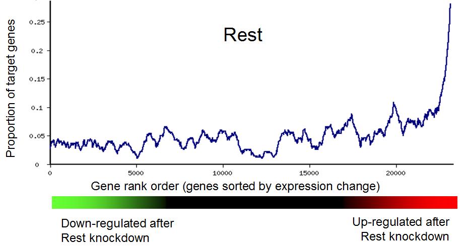 Fig. 3. Gene set enrichment analysis is used to generate a rank plot of the proportion of target genes of transcription factor Rest among genes that were downregulated and upregulated after the knockdown of Rest. If gene set enrichment is statistically significant (P ≤ 0.05) among upregulated genes, then some genes in the annotated gene-set are more abundant among upregulated genes than expected by random. However, PAGE does not provide information on the EPFP in these genes. Most studies of downstream effects of TFs assume that the set of regulated target genes is the intersection of two subsets: a subset of all target genes and another of genes that changed their expression following manipulation of a TF. However, the intersection may include a large number of false positive genes that change their expression not because of TF binding to promoters or enhancers but from other causes (e.g., second-order effects, compensation, etc.). Thus, a smaller subset of genes within the intersection needs to be delineated to bring EPFP below an acceptable threshold (Fig. 4). To identify enriched genes and evaluate their statistical significance by EPFP, users check a box "Identify associated genes" before doing gene set enrichment analysis. EPFP is calculated sequentially for different thresholds of gene expression change as a ratio of the proportion of targets among "control" genes (i.e., not affected by TF manipulation) to the proportion of targets among genes that responded to TF manipulation. The smallest fold change threshold that yields EPFP below the accepted level (e.g.EPFP ≤ 0.3), is then used to delineate the set of regulated targets of TFs.
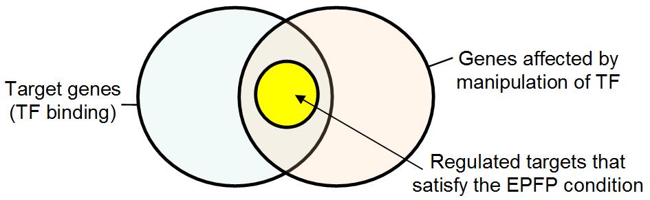 Fig. 4. Regulated targets of TFs represent a subset of genes within the set of common genes that are both TF tragets and upregulated (or dopwnregulated) after TF induction (or repression. Methods of gene set analyses described earlier assume that all genes in a set are equally weighted. However, experimental and mining methods used for generating gene sets often provide additional quantitative information for individual genes. Genes in a set may differ by z-score, p-value, expression change, number of sequence reads in ChIP-seq peaks, or in HITS-CLIP assay, and other criteria that may appear useful for the analysis of gene set enrichment. Thus, an option to handle gene sets with additional quantitative attributes was added to ExAtlas. If the box "Use attributes" is checked, then genes with low scores are transiently excluded from the analysis for varying score thresholds until the highest statistical significance (z-value) is achieved. This approach is applied both to gene set enrichment (PAGE) and to gene set overlap (hypergeometric test). The goal of meta-analysis is to use information from multiple independent studies to increase the power of statistical inference and reduce the number of false positives. ExAtlas applies four frequently used methods of meta-analysis: Fisher s, z-score, fixed effect, and random effect to evaluate the difference in gene expression between two Figure 4.6 Gene set enrichment scores (PAGE) for Gene Ontology (GO) annotated sets of genes among upregulated genes in mouse ESCs after induction of 137 individual transcription factors (TFs). Columns, induced TFs; rows, GO annotations. tissues or cell types. The first three methods assume that all studies implement exactly the same methodology (e.g., same cell lines, equipment, and reagents). In practice, however, methods often do not match between experiments, so the random effect seems to be most relevant method. Fisher s method combines log-transformed p-values from m studies and generates a chi-square statistic with 2*m degrees of freedom. The z-score method combines z-scores (i.e., the ratio of mean effect to its SD) of different studies with weights equal to square root of sample size. The fixed effect method estimates a weighted sum of effects (i.e., log ratio of gene expression change), where weights are equal to 1/σ2 with σ2 as the error variance. The random effect method takes into account the variance of heterogeneity between studies, T2, which is added to the variance of individual effects. Meta-analysis in ExAtlas starts by selecting gene expression data to be combined. Pairs of tissues (or cell types) are compiled from different data files or the same file. It is even possible to compile gene expression data from different species, and in that case, gene orthologs are compared. A list of all expression profile pairs used in meta-analysis can be saved for future retrieval and modification. The analysis is done using all four methods, and a table with the number of significantly overexpressed and underexpressed genes for each method is displayed. Differentially expressed genes can be saved as gene sets for functional annotation.
|