1. Introduction
ExAtlas is software for gene expression statistical analysis.
Main advantages of ExAtlas software for gene expression statistical analysis are the following:
- ExAtlas integrates all main functions for the analysis of gene expression data. Thus, there
is no need to move and reformat data between multiple applications.
- Supports data search and direct download of gene expression data (arrays and RNAS-seq)
from the GEO database
- Generates graphic and table outputs, including tab-delimited text tables
- Gene expression analysis is based on ANOVA (analysis of variance) of log-transformed values,
and includes multiple
options for error models that integrate error variances for multiple genes with a similar
expression level.
- Supports statistical analysis of gene expression data without replications, but this approach is
reliable only if the data includes a substantial number of samples.
- Supports pairwise comparison of expression profiles (p-value and false discovery rate - FDR),
principal component analysis (PCA), heatmaps, scatter-plots, bar charts, and 3D plots (VRML).
- Provides global analysis of two or multiple data sets, where all
components in data set A are compared/integrated with all components in data set B
- Includes analysis of global correlations between gene expression data sets and identification
of coregulated genes using Expected Proportion of False Positives (EPFP)
- Includes multi-profile gene set enrichment and gene set overlap tools based on EPFP and FDR
- Gene symbols and gene annotations are regularly updated from NCBI, ENCEMBL, MSIGDB and
other databases
- Several public data sets (e.g., GNF, BrainSpan, GO, KEGG, GAD phenotypes) are preloaded,
and updated regularly
- Every list of genes generated by the analysis or uploaded manually can be immediately used for plotting their
expression profile in any available gene expression data set and for functional annotation
by gene set overlap.
- ExAtlas has an online help page that provides with step-by-step instructions and annotated
screen captures.
The workflow in ExAtlas is shown below. Two main types of data files are gene expression
profiles and gene sets, which can be uploaded manually or retrieved from GEO database.
Tools for comparison of two or more data sets are shown as yellow boxes.
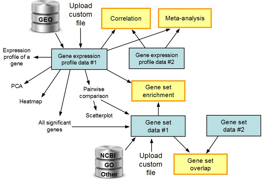
Fig. 1. The workflow in ExAtlas.
For example, a user may search GEO database for specific terms such as "kidney", "muscle", or
"T-cells", and the software provides information on samples where these terms are found. The
user then selects samples from the list and the software generates a gene expression profile data file.
ExAtlas can evaluate the quality of data and then low-quality samples can be removed. Alternatively,
expression profile data can be uploaded manually. The gene expression profile data
can then be used for ANOVA, pair-wise comparison between tissues or cell types, Principal
Component Analysis (PCA), making scatter-plots, expression profiles of individual genes, and
heatmaps. Several gene expression matrices are pre-loaded in the software as
public resources and are available to every user. Each gene
expression matrix can be compared using correlation analysis with any other expression matrix.
The main menu of the program (Fig. 2) includes buttons for various tasks, such as selecting the
organism species, Uploading new data files to ExAtlas, and retrieving gene expression data files
from the GEO (NCBI) database. The lower portion of the main menu is used to open various data
files as entry points to start the analysis, and refreshing file lists to show new files.
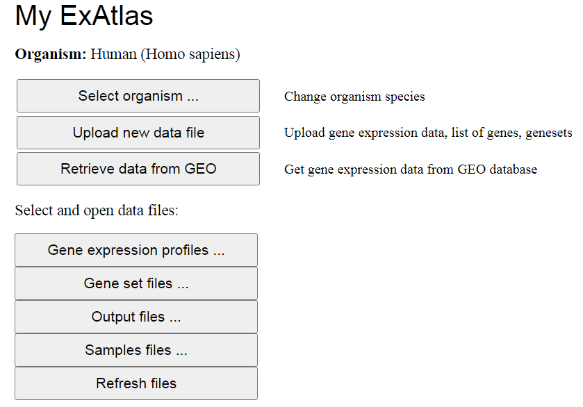
Fig. 2. The main menu in ExAtlas. Button name with dots
(...) indicates that clicking it opens a box dialog in the same page. Buttons without dots lead to
another page in the same tab or in a new tab.
There are four types of data files in ExAtlas, which can be accessed via four buttons in the main
menu. The first one is gene expression data file represented
by a table, where columns are samples and rows are either genes or microarray probes.
The second type of data is a gene set (or "geneset"), which is a set of gene symbols associated with
a certain biological function or certain pattern of expression (e.g., differentially expressed genes).
Some genesets carry additional information, such as score of individual genes or statistical
significance (e.g., FDR). Each geneset file usually combines multiple genesets. The ExAtlas software
stores many preloaded public geneset files, including Gene Ontology (GO), KEGG pathways, and BIOCARTA pathways.
The third type of data files is output, which is generated by various components of ExAtlas, such as
correlation analysis or geneset enrichment. Simple output files may include a single table of data,
but other output files include multiple tables of data. For example the correlation output includes
one table for correlation values, second and third tables show statistical significance (z-values and FDR),
and the fourth table is for lists of coregulated genes. Finely, the fourth data type is a list of samples
from one or multiple gene expression series in the GEO database. This data file is needed to generate a
combined gene expression data file.
2. How to use ExAtlas? Step-by-step instructions
List of tasks you can do with ExAtlas
- Open gene expression data and do statistical analysis (ANOVA)
- Search for a gene and display the expression profile for this gene
- Plot a heatmap for the gene expression profile data
- Principal Component Analysis (PCA)
- Pair-wise comparison of expression profiles of tissues or cell types
- Search GEO database and extract gene expression data
- Upload files for analysis: formats, normalization, editing, copying
- Generate a file with differentially-expressed genesets
- Correlation analysis between different gene expression data sets
- Exploring output files for correlation and other analyses
- Geneset enrichment analysis of up/down-regulated genes
- Meta-analysis
- Evaluate quality of individual samples and remove low-quality samples
- Exploring geneset files and/or analyze gene overlaps with another file
- Edit files
2.1. Open gene expression data and do statistical analysis (ANOVA)
If you click the button "Gene expression profiles" in the main menu (Fig. 2), a dialog box
appears where available gene expression files are shown in a drop-down list. Select a file and click
the button "Open data file"; then a new web page will appear which allows users to analyze
expression profiles in various ways (Fig. 3). If you open this file for the first time after uploading,
then you may need to wait till the statistical analysis is finished. If the data contains too
many columns, the interruption screen (Fig. 4) may appear while the analysis is performed.
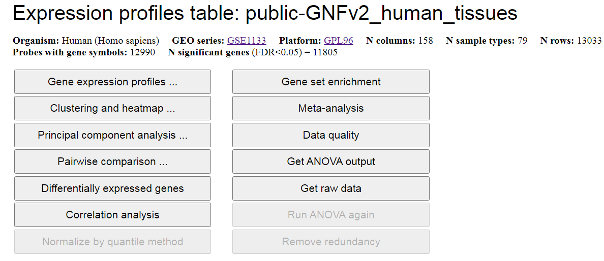
Fig. 3. Open expression profile matrix - screen capture.
From this screen you can generate expression profile (bar chart) of a specific gene,
plot a heatmap, do Principal Component Analysis (PCA), and do pairwise comparison of global expression
profiles for two kinds of tissues or cell types including a scatterplot that displays
differentially-expressed genes (DEGs). Other functions include generating DEGs for all pairs of
tissues or cell types (button "Differentially expressed genes"), correlation analysis, gene set enrichment
analysis, meta-analysis, evaluating data quality, downloading statistical
results (ANOVA), downloading raw data, normalizing data with quantile method
(
Bolstad et al., 2003), and removing redundant probes/gene symbols (leaving best probe or transcript
for each gene).
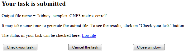
Fig. 4. Interruption screen is used for long computational tasks.
Statistical analysis of gene expression data is based on the single-factor ANalysis Of VAriance
(ANOVA). The program calculates F-statistics which
is a ratio of factor variance (i.e., variance between averages for factor levels) to the
error variance. F-statistics is then used to estimate the P-value
according to theoretical F-distribution. Because ANOVA is done simultaneously for several thousands of
genes, it is necessary to adjust results for multiple hypotheses testing.
The False Discovery Rate (FDR) shows the expected proportion of false
positives among genes that are considered significant; it is estimated from p-values using the method
of Bejamini-Hochnberg. FDR ≤ 0.05 and fold change ≤ 2 are used as default criteria of statistical
significance. The error model attempts to get a better estimate for the true error variance than
the error variance estimated from data (we call it 'empirical error variance').
In ExAtlas, we use the maximum of empirical error variance and error variance averaged across 500 genes
with similar average expression. This error model is proposed by
Sharov et. al. (2005) as
a method to reduce the number of false positives. ANOVA output file is downloaded after clicking the button
"Get ANOVA output (Fig. 3).
Additional options for running ANOVA are available if you chose to "Run ANOVA again" and click the
button with this name in the menu (Fig. 3). In the figure, this button is grayed (disabled) because
this particular file is public and its analysis can be modified only by the administrator.
However, you can make your own copy of public data (as explained below), and then run ANOVA with custom
parameters or with a custom annotation file for the array platform. When running ANOVA again you
can select one of the following error models:
- = Actual error variance for each probe,
- = Average error variance for probes with similar expression level,
- = Bayesian correction of error variance (Baldi & Long 2001),
- = Maximum between actual and expected average error variances,
- = Maximum between actual and Bayesian error variances.
In addition, you can select a cutoff expression value (probes with maximum value below cutoff are ignored), modify
the threshold z-value used to remove outliers, modify proportion of probes with high error variances
to ignore in error models, or modify the number of probes in a sliding window to average error variance.
With ExAtlas, users can run ANOVA-like analysis even for data sets with no replications
(this option is usually not available in other software). In this case, the error variance
is estimated based on the half-normal probability plot method. We assume that at least
a half of degrees of freedom in a set of gene expression values
represent random effects. Thus, the standard deviation, σ, of random effects can be
approximated by the median of positive deviation (i.e., absolute value of deviation) from the
mean divided by 0.675 (inverse half-normal cumulative distribution for p=0.5). The error variance in ANOVA is then set to σ2.
This method is applied to each set of the 500 genes in a sliding window that is shifted
across the set of all genes sorted by their average log-expression. This error variance is
then used for evaluating the significance of gene expression change in individual genes.
2.2. Search for a gene and display the expression profile
Click the button "Gene expression profiles" in the menu on Fig. 3 to open the dialog box (Fig. 5), where you can enter
a gene symbol (or GenBank accession or array probe ID in the field "Search term" and specify the type
of search term using the pull-down list and click the button "Search".
If many genes (or probes) match to your search, all of them
will be displayed, and then you can select individual genes or probes. Checkbox "Sort" can be checked
if you wish to sort tissue or cell types by decreasing order of expression value. When the gene
(or probe) is found, ExAtlas generates a histogram with gene expression profile (Fig. 6),
and a table of expression in each tissue/cell type. The histogram shows average log-expression values
for each cell type or tissue; to see values for individual replications
click the button "Show replications".
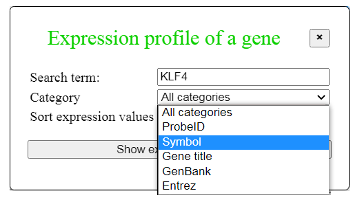
Fig. 5. Dialog for finding expression profile of a gene
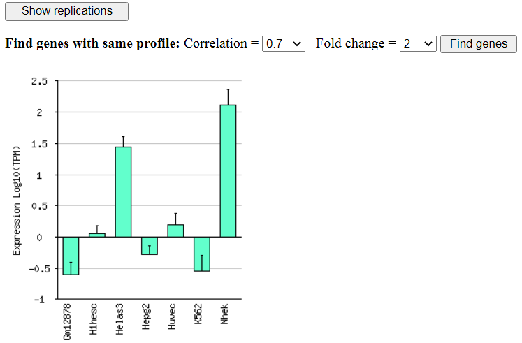
Fig. 6. Expression profile of KLF4 in various human cell lines (ENCODE GSE23316)
From the screen with gene expression histogram (Fig. 6) you can search for other genes with a similar
expression profile using correlation threshold and fold change threshold.
2.3 Plot a heatmap for the gene expression profile matrix
To plot a heatmap, click "Clustering and heatmap" button in the menu (Fig. 3) to open a dialog box
(Fig. 7), where you can select gene filtering parameters (FDR threshold
and fold change threshold), and the type of filtering and clustering. You can check the box
"Show replications" if you want to see data for individual replications. Then click the button "Make heatmap",
and the heatmap will appear in the new tab (or new screen) of the browser (see example in Fig. 8).
Because of the
large number of genes, gene symbols on the left are not visible and are represented by gray area (or lines).
However, if you click in the row header area, gene name and expression profile are displayed at the left
corner of the screen.
Filtering of genes is important, to save processing time, and to reduce the complexity of the heatmap.
Non-significant genes only add noise to the heatmap, and better
filtered out. After the heatmap is displayed,
you can download the filtered and sorted matrix (as a tab-delimited text file) by using the link
"Matrix file" at the top of the page. This file can then be examined in Excel.
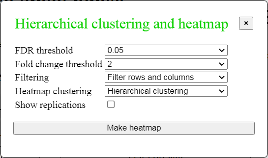
Fig. 7. Dialog box to make a heatmap
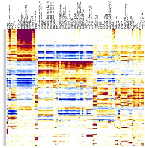
Fig. 8. Example of a heatmap for GNF mouse v.3 data
The bottom portion of the screen with the heatmap is designed for editing. To change color intensity,
you can change the maximum value and click "Re-plot the matrix" button. Also, you can delete of move
columns and rows using menu fields.
2.4. Principal Component Analysis (PCA)
To start PCA, click the button "Principal component analysis" in the menu on Fig. 3. A dialog box will
appear (Fig. 9), where you can select gene filtering parameters (FDR threshold
and fold change threshold), type of filtering, and a check box to show replications.
Another check box can be used to add analysis of PC-related gene clusters; if it is selected, then two
other parameters are utilized: cluster correlation and fold change thresholds.
Click the button "PCA analysis" to start the process. PCA is computed using the Singular Value Decomposition
method that generates eigenvalues and eigenvectors both for rows and columns of the log-transformed
data matrix. For plotting of rows and columns together (biplot) we used column projections
(Gabriel 1971,
(a href-https://academic.oup.com/bioinformatics/article-pdf/24/24/2832/49056337/bioinformatics_24_24_2832.pdf>
Chapman et al. 2002).
The advantage of the biplot compared to a traditional PCA is that the user can visually explore associations
between genes and tissues. ExAtlas generates 2-dimensional and 3-dimensional
(based on VRML) biplots (Fig. 9). All biplots (including 3D) are interactive; each gene is
a hyperlink to its annotation and expression pattern. To view PCA in 3-dimensions you need a VRML
viewer, for example FreeWRL or Cortona3d.
Fig. 9. PCA and biplot of mouse gene expression in various tissues (GNF database).
A and B = 2-D biplot for tissues and genes, respectively; C = 3-D PCA; D = 3-D biplot for
tissues (green spheres) and genes (blue cubes).
If "PC gene clusters" option is chosen, then clusters of genes are identified that are
positively and negatively correlated with each principal component (Fig. 10). The degree of gene
expression change within a specific PC is measured by the slope of regression of
log-transformed gene expression versus the corresponding eigenvector multiplied by the
range of values within the eigenvector. Gene is associated with the most correlated PC;
however two additional conditions should be met: (a) the degree of gene expression
change exceeds the fold change threshold, and (b) the
absolute value of correlation exceeds the correlation threshold).
Fig. 10. Gene clustering based on principal components
2.5. Pair-wise comparison of expression profiles of tissues or cell types
Click "Pairwise comparison" button in the menu on Fig. 3 to open the corresponding dialog box (Fig. 11),
which allows to select tissues or cell types to be compared, FDR threshold, fold change threshold, and minimum
gene expression threshold. In addition, median gene expression value can be used as a baseline for comparison.
All replications are averaged as a default, but it is still possible to analyze
individual replications by selecting replication in a pull-down menu on the right
Start the analysis by clicking the button "Scatter-plot and statistical significance".
In the scatterplot (Fig. 12),
each point represents one gene with coordinates equal to log10 expression in each tissue or cell type
in TPM units. Gray dots represent non-significant genes, red dots = significant
upregulated genes, and green dots - significant downregulated genes. Statistical significance is
based on error variance estimated with ANOVA.
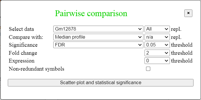
Fig. 11. Dialog box for pairwise comparison.
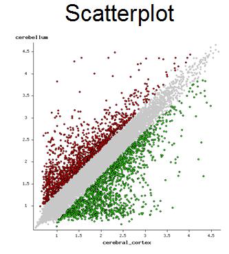
Fig. 12. Scatter-plot of gene expression in two cell lines (ENCODE GSE23316)
To display the list of significant genes click on the link "List of over-expressed genes" or
"List of under-expressed genes". A new web page appears in the next tab where you click on gene symbol
(or probe ID) to get the expression profile of that gene. The list of genes can be downloaded as a
tab-delimited text file. It can also be used for functional annotation (e.g., GO, KEGG), and for plotting
their gene expression in the form of heatmaps.
If you use median expression profile for comparison (as control)
then an additional feature is recorded in the output table: a z-value that characterizes gene
specificity (column header "Specificity"). This z-value is estimated
by comparing log-expression in a given tissue (mi) with the average expression in other
tissues (M) that are not correlated with this tissue
(see details here).
2.6. Search GEO database and extract gene expression data
Click the button "Retrieve data from GEO". A new web page appears, where you type in comma separated
search terms (e.g., iPSC, astrocytes), terms to avoid (e.g., patient, cancer, tumor, carcinoma, biopsy, diabetes),
and platform. Search terms can include specific GEO series ID (e.g., GSE3526, GSE18959). In this case,
only these series are displayed. Two types of data can be extracted from GEO:
expression profiling by microarrays
(arrays) or RNA-seq. You can select a specific array platform to ensure compatilibility of
multiple gene expression data sets. Only a small portion of RNA-seq data is available for direct retrieval
from GEO - only those samples that have been processed by NCBI. Other RNA-seq data can be uploaded
manually, as explained in the following section.
There are two options to present results of GEO search: showing all individual samples or showing only
series of data. In the latter case, you include all samples from each selected series of data.
But you will still have a chance to remove extra samples at the following step after you save the list
of all selected samples.
After you click the "Search" button, a new page with serach results will appear. Results may include
multiple pages, where you need to select those samples in which you are interested. Sample selection
is retained when you move from one page to another. After all samples are selected, specify the file
samples name. You can accept the proposed file name or modify it as necessary. Then you click the button
"Save samples" and a new page will appear with the list of samples. You can keep editing this list
by removing or adding samples. Also you can modify the names of samples to make them more informative
for future use. Samples within the same series and having identical names are interpreted by ExAtlas
as replications. Thus, you need to delete replication information from sample name. For example,
if the sample is named: "Hela cells untreated, rep2", you need to delete the ending ", rep2".
After the list is finalized, generate a
combined matrix of all samples by clicking the button "Generate matrix". Although samples from
different data series (GSE accession numbers) can be combined in one list of samples, in many cases
it is better to save each data series separately, upload corresponding data from GEO, and later
combine data series using batch-normalization method (see Edit files).
Downloading and processing the data takes some time. Thus, the "interruption screen" appears
(see Fig. 4). In this window you can check the status of your task (use te link to "Log file"),
cancel the task, or close the window without cancelling the task.
Keep reloading the log file to see changes. If you click "Check your task" but it is not finished,
then the screen will say "Your task is not finished!" Results will be shown when the task is
finished. If data comes from different array platforms, expression profiles are combined based on
gene symbol, and if multiple probes are available for a gene, then the best probe is used with
either higher statistical significance (F-statistics) or higher average signal intensity (if there
are no replications). However, if all samples are obtained with the same array platform, then
redundant probes are not removed; and thus, a gene can be represented by multiple probes.
If you cannot find a specific data set, which you know exists in GEO, this may have resulted from
data filtering. Your data set may have been filtered out because the array platform type
is a cDNA array, tiling array, genomic array, exon array, non-matching species.
However, if you download the gene expression data manually then you can upload it
using "Upload new data file" button in Fig. 2.
2.7. Upload files for analysis (formats, normalization, etc.)
The "Upload new data file" button in the main menu (Fig. 2) is used to open the screen for
file upload (Fig. 13). You either browse for the file to be uploaded (button "Choose file") or paste the
text file into the provided text area. Then, select the type of file (i.e., Gene expression
profile matrix, Gene set file, Samples file, List of geneset, Output file, or Annotation file).
If you want to store the file under different name, type-in the file name in the "Rename file as:"
field. Filling up file description is optional. If the file with gene expression profile table does not
include information on array platform, then you need to select the platform.
If the array platform is not present in the pull-down menu list, you need to upload a file with
platform annotation which should include at least 3 columns: "probe ID", "gene symbol", and "gene name".
You can add more columns that specify GenBank accession numbers, Entrez ID, or Unigene ID.
If gene symbols or GenBank accession numbers are used in the first column of the gene expression data file,
then select "Gene symbols" or "GenBank" platform, respectively.
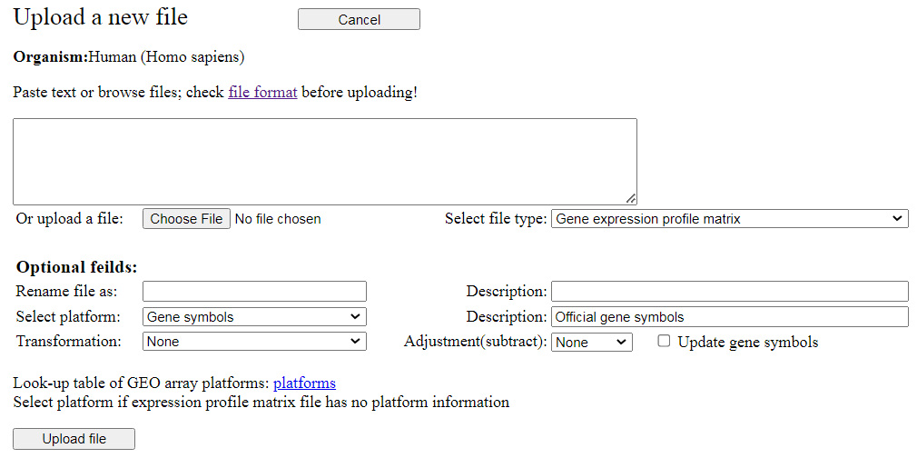
Fig. 13. Screen for uploading custom data files.
Here is a brief description of file formats.
The gene expression profile is a tab-delimited text that follows MIAME standards. All array matrix
files downloaded from GEO can be directly uploaded to ExAtlas. The file has header lines that
start with "!" sign. However, these lines are optional. You can upload a file even without these
lines if you specify platform for the gene expression profile file and in column headers are informative.
Header lines are followed by a table with data lines that specify the intensity of feature
signals. Here is an example of a gene expression profile matrix file:
!Series_title	"Gene expression of human soft tissue sarcoma"
!Series_geo_accession	"GSE2719"
!Series_pubmed_id	"15994966"
!Series_summary	"Gene expression profiles of 39 human sarcoma samples (GSM 52571-GSM52609)..."
!Series_type	"Expression profiling by array"
!Series_platform_id	"GPL96"
!Series_platform_taxid	"9606"
!Series_sample_taxid	"9606"

!Sample_title	"brain"	"stomach"	"colon"	"pancreas"	"prostate" ...
!Sample_geo_accession	"GSM52556"	"GSM52557"	"GSM52558"	"GSM52559"	"GSM52560" ...
!Sample_taxid_ch1	"9606"	"9606"	"9606"	"9606"	"9606" ...
!Sample_data_row_count	"22283"	"22283"	"22283"	"22283"	"22283" ...
!series_matrix_table_begin
"ID_REF"	"GSM52556"	"GSM52557"	"GSM52558"	"GSM52559"	"GSM52560" ...
"1007_s_at"	2867.1	1780.8	1921.8	2486.1	4151.4	...
"1053_at"	216.4	196.8	145.3	127.1	109.7	...
"117_at"	135	121	157.2	162.6	267.8	...
"121_at"	916.1	1075.7	922	2192.9	1198.8	...
"1255_g_at"	149.8	35.5	32.7	96.3	47.6	...
..................................................................
!series_matrix_table_end
Sample names are taken from the line "!Sample_title" or from the line of column headers that follows
after "!series_matrix_table_begin". Column headers for replication samples should be exactly matching
(case-sensitive). It is not required to reorder columns so that all replications are placed together;
replicetion samples are recognized by column headers even if they are separated by other samples in
the table. ExAtlas can process 2-dye arrays that use reference RNA consistently as one of the
channels (e.g., Cy5 or Cy3). In this case, two columns that correspond to the same array (channel #1
and channel #2) should be placed together and the column representing reference RNA should be named
"reference". If data are log-transformed or Z-value transformed, then select transformation type from
the pull-down menu.
Because background subtractions may result in negative values, some array scanning programs avoid
negatives by adding some constant value to signal intensity (e.g., 50 or 100). Usually this does not cause problems,
but low-expressed genes may show weaker expression fold-change. If you would like to remove this
constant value, then select "adjustment" value from the pull-down menu.
Alternatively you can compile gene expression data column-by-column from one or multiple tab-delimited
text tables. To use this option, select "Compile expression profile" option from the
pull-down list "Select file type:". Type-in file name in the field "Rename file as" and
description. Select array platform if applicable, then browse to select the first data
table and click "Upload" button.
After the table is parsed and column headers displayed on the screen,
select columns to be extracted, specify their usage (Probe ID/tracking ID, Gene ID/name,
or Gene expression), and possibly edit column header.
If you have specified array platform, use column with probe ID as "Probe/tracking ID".
Alternatively, select a column as Gene ID/name if it has gene symbols, GenBank acc.,
Entrez gene ID, or Ensembl gene ID. Please, edit column headers as 'symbol', 'refseq', 'genbank', 'entrez',
or 'ensembl'. Probe/tracking ID or Gene ID/name
should be common for all data files that are assembled together. When these data are uploaded,
you can choose another data table and extract data from it until all data are compiled.
It is necessary to specify Gene ID/name at least in one of the tables. For example you
can upload an annotation table where both Probe ID/tracking ID and Gene ID/name are
present. At any time you can edit sample names to make them meaningful and ensure that
replications have exactly the same sample names (case-sensitive). If you have 2-dye arrays
and one channel is used for reference RNA, then edit column name as 'reference'. In this case,
reference expression is used for normalization as follows: norm(x) = x*My/y, where x is
signal intensity for sample, y is signal intensity for reference, and My is geometric mean
of all reference values.
In a geneset data file (tab-delimited text), each line corresponds to one geneset.
First item in the line is geneset ID, the second is geneset description (which may be blank or duplicate ID),
followed by all genes that belong to this geneset. Because
some lines are rather long, geneset files may not always be opened in Excel.
Geneset file may include header lines that all start with "!". Here is example of a geneset file:
CITRATE_CYCLE_TCA_CYCLE	CITRATE_CYCLE_TCA_CYCLE	Idh3g	Pdha2	Fh1	Suclg1	Idh2	Pcx	Pdha1	Idh3b	Sucla2	Mdh1	Suclg2 ...
ETHER_LIPID_METABOLISM	ETHER_LIPID_METABOLISM	Pla2g4e	Pla2g7	Pla2g12a	Pla2g4a	Lpcat4	Agps	Pafah2	Pla2g3	Pla2g2f	Ppap2a ...
..........................................................................................................
An alternative acceptable format of geneset files uses comma-separated lists of gene symbols:
CITRATE_CYCLE_TCA_CYCLE	CITRATE_CYCLE_TCA_CYCLE	Idh3g,Pdha2,Fh1,Suclg1,Idh2,Pcx,Pdha1,Idh3b,Sucla2,Mdh1,Suclg2,...
ETHER_LIPID_METABOLISM	ETHER_LIPID_METABOLISM	Pla2g4e,Pla2g7,Pla2g12a,Pla2g4a,Lpcat4,Agps,Pafah2,Pla2g3,Pla2g2f,Ppap2a,...
..........................................................................................................
Sample files (tab-delimited text) have 4 columns:
(1) series ID from GEO, (2) Platform ID, (3) Sample ID, and (4) sample title/name. Samples
with identical titles within the same data series are considered as replications. Check title
spelling, spaces, and character case, because in the case of mismatch replications will not be
recognized. Example:
GSE6290	GPL1261	GSM144590	renal corpuscle
GSE6290	GPL1261	GSM144591	renal corpuscle
GSE6290	GPL1261	GSM144594	Early Proximal Tubule
GSE6290	GPL1261	GSM144595	Early Proximal Tubule
GSE6290	GPL1261	GSM144596	Medullary Collecting Duct
GSE6290	GPL1261	GSM144597	Medullary Collecting Duct
GSE6290	GPL1261	GSM144603	s-shaped_body
GSE6290	GPL1261	GSM144604	s-shaped_body
GSE6290	GPL1261	GSM144605	s-shaped_body
............................................................
Annotation file has at least 3 columns: (1) Probe ID, (2) Gene symbol, and (3) Gene
name. Additional columns may show accession number, Entrez, Ensembl, Unigene or other IDs.
Do not use multiple gene symbols in the second coumn! If a probe matches to multiple symbols
then select the best symbol for annotation. If you need to show other matching gene symbols,
then make multiple copies of the line with this probe ID in the gene expression profile data
and modify probe ID (enter unique new ID) which will be associated with alternative symbols.
Annotation file always has a line with column headers and may include optional header lines
that start with "!".
NIA-oligo	Gene symbol	Gene name	GenBank	Entrez
Z00000225-1	Wdr74	WD repeat domain 74	NM_134139.1,NM_134139.1	107071
Z00000233-1	Tro	trophinin	NM_001002272.2,NM_001002272.2	56191
Z00000238-1	Edf1	endothelial differentiation-related factor 1	NM_021519.1,NM_021519.1	59022
Z00000241-1	Pfn1	profilin 1	NM_011072.2,NM_011072.2	18643
Z00000244-1	Rabep1	rabaptin, RAB GTPase binding effector protein 1	AK163126.1,AK163126.1	54189
.........................................................................
Output files may include one or several tab-delimited tables. When you perform any
analysis in ExAtlas (correlation, gene enrichment, significant genes, etc.) you can
then download the output file to explore its format. Any tab-delimited table with first line
of column headers and with the first column as row headers can be uploaded as output file
for plotting as a heatmap. No additional formatting is needed.
Lists of genes (official gene symbols) can be uploaded to explore the enrichment of
various genesets for functional annotations (e.g., for comparison with GO-terms, KEGG pathways).
Genes can be formatted in one column or pasted as comma-separated text.
After the list of genes is uploaded, select the geneset file for comparison (e.g.,
GO_mouse_geneset), specify parameters (FDR and fold enrichment) and click "Enrichment analysis".
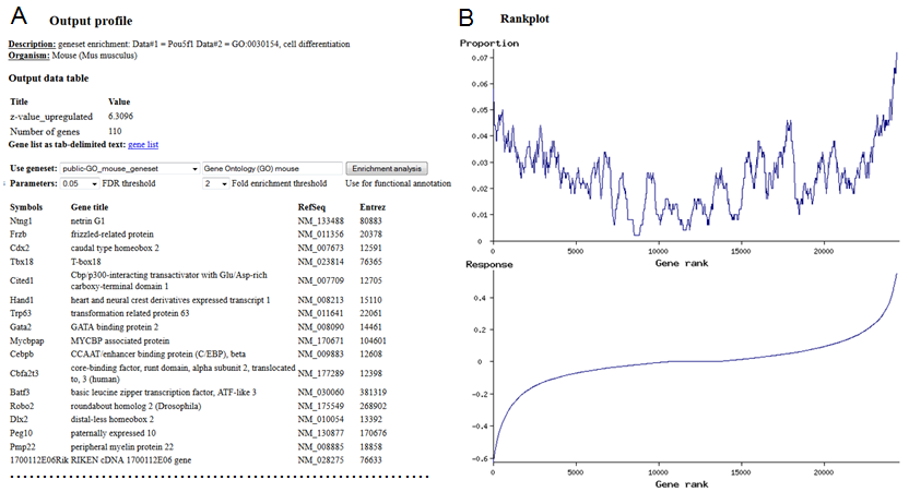
When the output opens, click on the button "Get profile".
2.8. Generate a file with differentially-expressed genesets
ExAtlas automates the generation of genesets of upregulated and downregulated genes, which can
be later used for comparison with other data sets. Expression of each gene is compared to the
baseline expression, which can be either a median (default) or expression
in some specific tissue/organ or cell type. Conditions of
statistical significance are defined by FDR threshold and fold change threshold. Aa additional
condition is gene specificity that allows users to narrow down the list of genes to specific genes.
Specificity is measured by z-value, as explained in the pair-wise comparison
section. To select highly-specific genes use z-values ≥ 6. Consider editing the name and
description of the output geneset file before starting the task, then click the button "Save
significant genes". When the task is finished, the output file displays a histogram of the number
of significantly upregulated (orange) and downregulated (dark blue) genes.
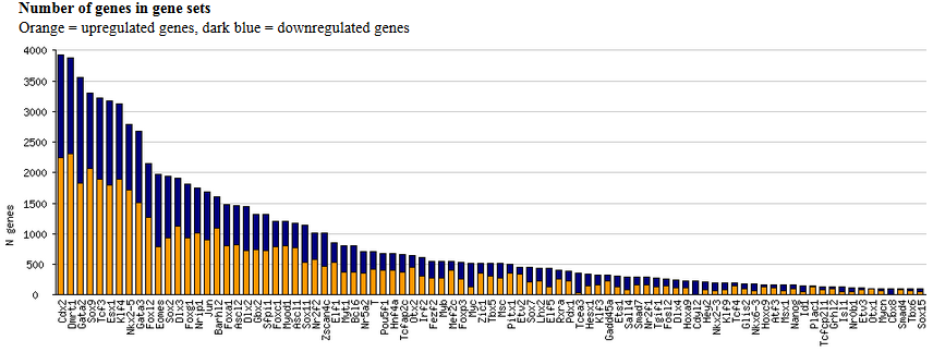
Fig. 16. Histogram of the number of significantly upregulated (orange) and downregulated (dark blue) genes
after the induction of various transcription factors in mouse ES cells.
2.9. Correlation between different gene expression data sets
To characterize the effect of treatments on gene expression profiles it is often necessary to
examine correlations between different gene expression data sets. For example, the change of
expression of genes following the induction of various individual transcription factors in ES
cells was compared with gene expression profiles in various tissues and cell types
(Nishiyama et al. 2011 and
Nakatake et al. 2020).
Results indicate
that some transcription factors (e.g., ASCL1, GATA3, MYOD1, SPI1) induce tissue-specific genes.
To estimate correlations, first open the file with gene expression profiles, then click the
"Correlation" button in the menu shown in Fig. 3. This will take you to the next
screen where you can select the second file with gene expression profiles (Fig. 10). If you need
an autocorrelation analysis, use the same file as #1 and #2. If you want
to compare gene expression change between different species, then change the species
for comparison. The screen will be reloaded with a list of data for another species. Use FDR threshold
and fold change threshold to limit the number of genes. Lower values of FDR and higher values of
fold change correspond to more stringent filtering.
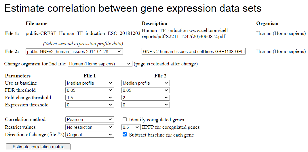
Fig. 10. Screen for correlation analysis of two data sets with gene expression profiles.
The algorithm for estimating correlations is the following.
- Log-transform gene expression data and run ANOVA for each file
- If there are multiple probes in array for the same gene, select the best probe (with highest F).
- In each file, select significant genes based on FDR and fold-change thresholds
- Find common genes that are selected for both files - these genes are used for estimating correlations
- Subtract median expression value (or other baseline, e.g., control sample) in each row.
Because all expression values are already log-transformed in ANOVA, the subtraction yields a logratio value
- Take column i from the first matrix and estimate its correlation (Pearson or Spearman) with the column j in the
second matrix. This correlation value is placed in column i and row j in the output table.
All these steps are done automatically after you click on the button "Estimate correlation matrix".
Before you start the task, specify the output file name and its description (edit suggested name).
Because estimating correlations usually takes several minutes, an interruption web page appears
where you need to check the status of your task.
If you check the box "Identify coregulated genes", then ExAtlas will identify lists of genes that
are both upregulated or both downregulated in two data files if correlation is positive and
significant (z ≥ 2), and Expected Proportion of False Positives (EPFP)
is smaller than the specified threshold (0.5, by default).
The algorithm for finding positively
coregulated genes is based on the analysis of data points in the positive quadrant (i.e. x>0 and y>0).
Negatively coregulated genes are identified in the same way in the negative quadrant. First, logratios
of gene expression change are all replaced by their ranks. If the null-hypothesis is true (no correlation)
then the genes are expected to have a uniform random distribution in the positive quadrant (Fig. 11A).
To estimate EPFP for a gene with rank rx in the first expression profile (file #1) and rank ry in the first
expression profile (file #2), we estimate the density of dots/genes in a rectangle with lower left corner at
(rx,ry) coordinates (Fig. 11B, dark-shaded area) and compare it with the density of dots in two adjacent
rectangles to the left and down (light-shaded areas). EPFP equals the density of dots in the light-shaded
divided (which serves as a baseline) by the density of dots in the dark-shaded area. Because we have two
light-shaded rectangles, EPFP is estimated twice, and then we select the larger value (to be conservative
in our assessment). Because EPFP may not monotonically decrease with increasing rank rx and ry, it is forced
to decrease monotonically. In particular, if EPFP(rx1,ry1) > EPFP(rx,ry), and rx1 > rx, and
ry1 > ry, then EPFP(rx1,ry1) is set equal to EPFP(rx,ry).
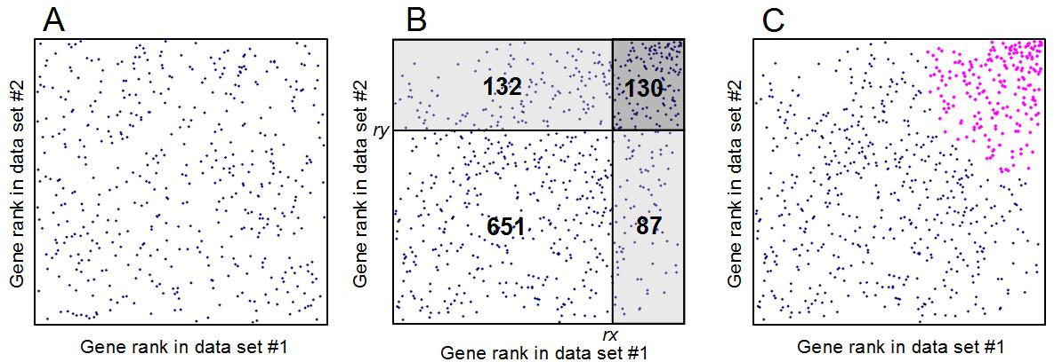
Fig. 11. Estimating Expected Proportion of False Positives (EPFP)
for coregulated genes: (A) scatter-plot of gene expression rank in the positive quadrant if there is no
correlation. (B) The same plot if gene expression profiles are correlated, numbers indicate gene counts.
The density of dots/genes in the dark-shaded rectangle, 130/(132+130)/(130+87)=0.002287, is compared with
the density of dots/genes in two light-shaded rectangles: 132/(132+130)/(132+651)=0.000643 and
87/(651+87)/(130+87)=0.000543. Two estimates of EPFP are generated for the gene at the low left corner of
the dark shaded rectangle (with expression ranks rx=651+132=783 and ry=651+87=738):
EPFP1 = 0.000643/0.002287 = 0.281 and EPFP2 = 0.000543/0.002287 = 0.237. The greater value is
selected: EPFP = 0.281. (C) All coregulated genes with EPFP≤0.3 are highlighted (magenta).
To identify oppositely coregulated genes (i.e. upregulation in file #1 associated with downregulation in
file #2 and vice versa), set "Direction of change (file #2)" to "Reversed" (Fig. 10). Then
gene expression change for File #2 is inverted (multiplied by -1).
2.10. Exploring the output file
When the output table for correlation analysis is generated, results are saved in the output file,
which is opened automatically. Output files can be saved and opened manually later from the main menu
(Fig. 2). When the output file screen is displayed (Fig. 12), then it can be used to
plot the full output table as a heatmap (section #1) or to plot bar charts for rows and columns
of the output table (section #2). Examples of output graphs are shown in Fig. 13.
Plotting options depend on the type of analysis and usually include z-values, which indicate
the statistical significance of correlation. In addition, correlation values and/or the number of
associated genes is provided. After you selected which table to plot, click the button
"Plot output table". You can also plot profiles for individual rows and columns of the
output table by selecting respective rows or columns in section #2 "Profiles of rows,
columns, and cells". Values are sorted in profiles from high to low because sorting is convenient
for functional annotations of genes (e.g., by Gene Ontology or pathways).
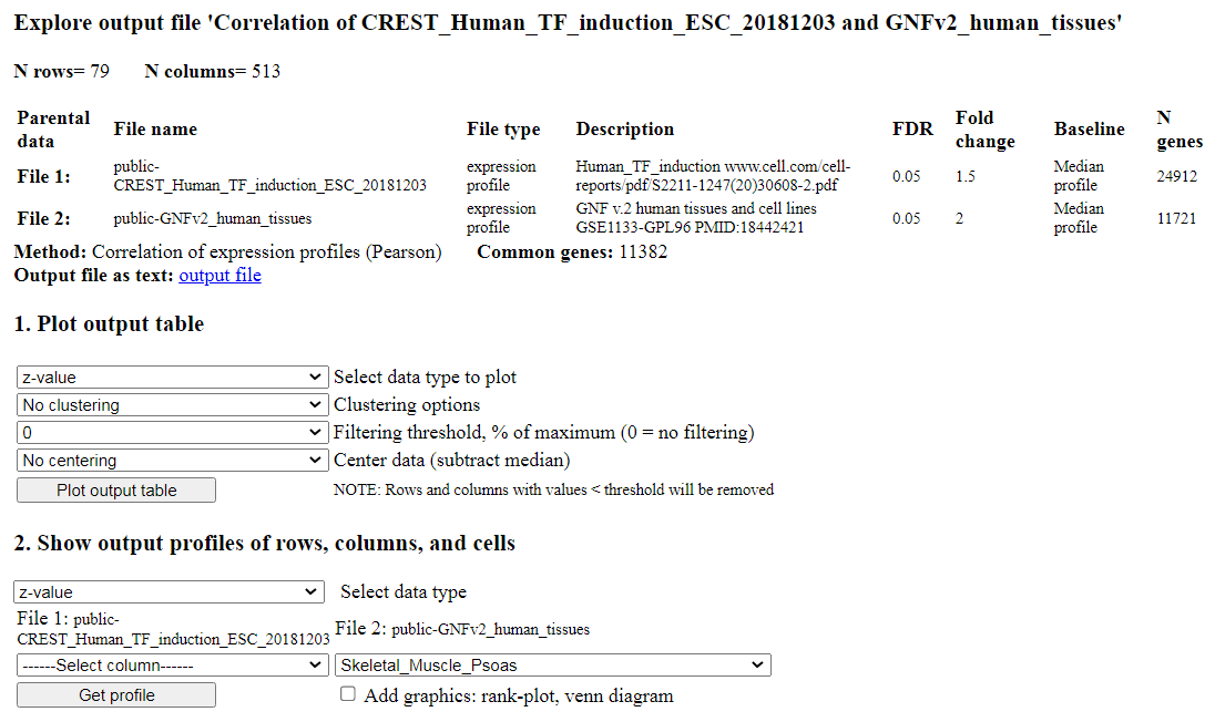
Fig. 12. Open output file screen: results of correlation analysis.
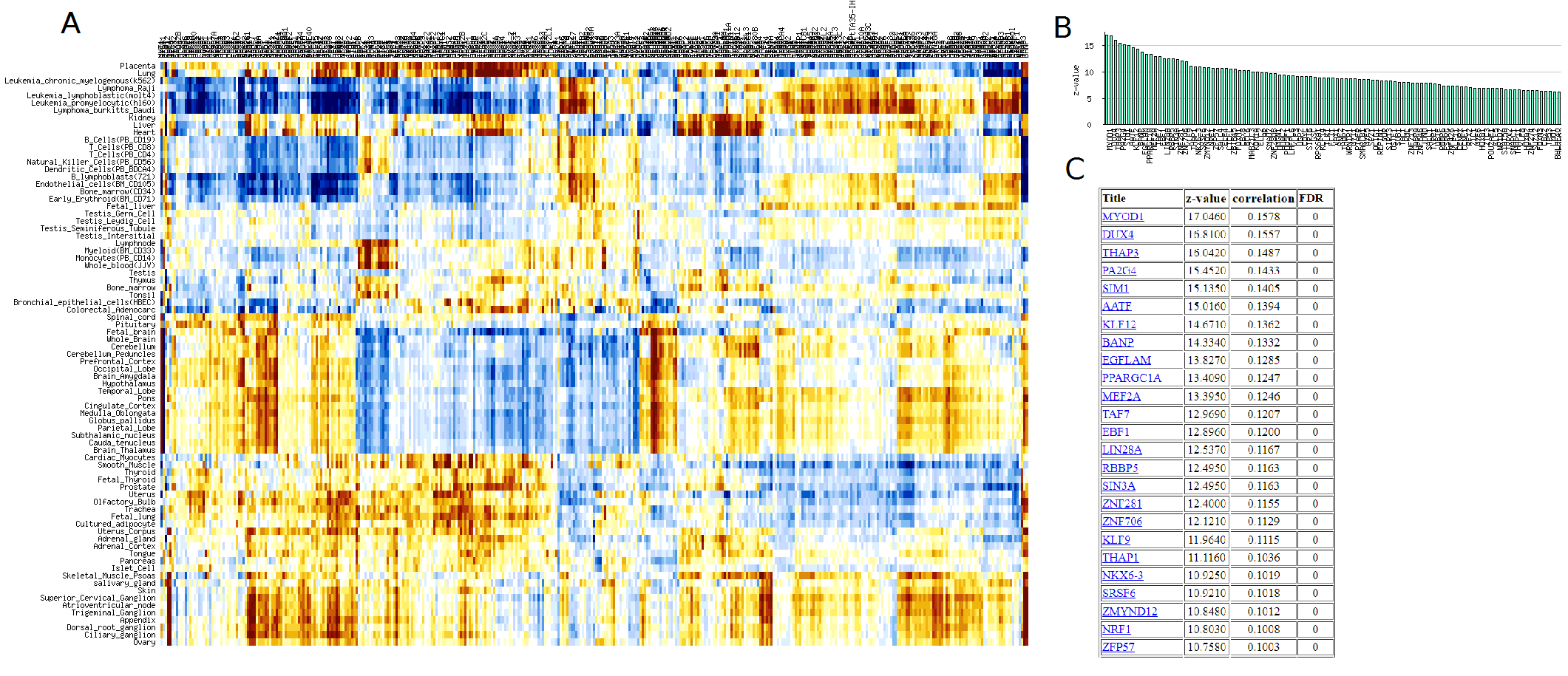
Fig. 13. Example of correlation matrix (A), profile for a single row (B), and table of
transcription factors
with highest correlation with gene expression in skeletal muscles (C).
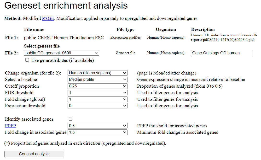
2.11. Geneset enrichment analysis of up/down-regulated genes
Geneset enrichment analysis is used to evaluate if specific genesets (such as Gene Ontology
or KEGG pathways) are over-represented among upregulated and/or downregulated genes. The
advantage of geneset enrichment analysis compared to a simple overlap of
genesets is that no thresholds are used for selecting differentially expressed genes.
In particular, geneset enrichment analysis can find significant associations with functional
genesets even if there are no significantly upregulated genes based on standard criteria
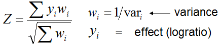
(e.g., FRD $le; 0.05 and change ≥ 2 fold). Among various existing methods for geneset
enrichment analysis we use Parametric Analysis of Gene Enrichment (PAGE) (Kim & Volsky 2005, PMID:15941488)
because of its simplicity and reliability (Zhang et al. 2010, PMID: 20092628). PAGE is based
on the comparison of the average expression change in a specific subset of genes,
xset, with the average expression change in all genes, xall:
To start PAGE analysis, select the geneset file using pull-down list (Fig. 14). To use
geneset file for a different species, first select species. The screen will be reloaded with a
list of data for that species; after that select the geneset file.
To identify associated genes (e.g., target genes with binding sites of transcription factor which
at the same time responded to the induction or knockdown of the same transcription factor) check
the box "Identify associated genes". Use EPFP threshold and fold change threshold to limit the
number of associated genes. Lower values of EPFP and higher values of fold change correspond
to more stringent filtering.
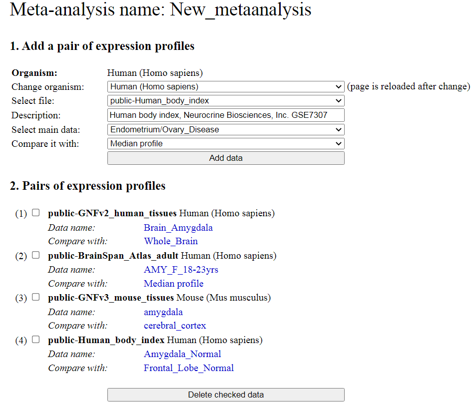
If all data sets use the same array platform, then the meta-analysis is done for each probe ID
(there may be multiple probe ID-s for the same gene). Otherwise, the meta-analysis is done
for each gene symbol. If some data set belongs to a different species, then gene symbols are
converted to the homologs in the first species
using HomoloGene. To delete
a data pair, use the corresponding checkbox and then click on the button "Delete checked data".
Part 3 in the menu (Fig. 9) allows users to save meta-analysis design for the future: click on
the button "Save metaanalysis". Also you can load one of the previously saved meta-analysis
designs: select the file you need and click the button "Load metaanalysis".
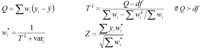
When all data sets for meta-analysis are assembled, select parameters for meta-analysis
(FDR threshold and fold-change threshold), and click the button "Start analysis". The
output page shows the number of significant genes for each method of meta-analysis. Click
on the number of gene to display the list of genes and corresponding statistics. Effects are
shown as either logratio (log10) (default) or as fold change. The format of effects can be
selected above the output table that shows the number of significant genes for each method.
The list of significant genes can be further explored for significant overlap with various
data sets.
2.13. Evaluate quality of samples and remove low-quality samples
Click the button "Data quality" near the bottom of the "Open expression profile" screen (Fig. 4) to
run quality control program. If the data file is large, the interruption screen (Fig. 4) may
appear as discussed above. Quality control checks (a) correlation of log10-transformed expression
of housekeeping genes with standard data (RNA-seq), and (b) consistency between
replications. Consistency of replications is assessed by modified standard deviation (SD) of
the log-transformed expression in each sample from the tissue-specific median (where outliers with
z > 3.5 are not used for estimating median). In general, SD < 0.1 means good quality, and
SD > 0.3 means bad quality. Correlation of expression of housekeeping genes usually is in the
range from 0.5 to 0.95. If it falls below 0.5, then the quality may be low. Checkboxes
located near each sample allow the user to select samples with low quality for deletion.
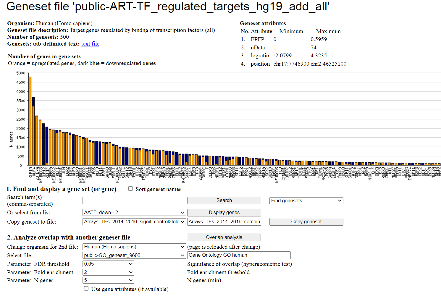
This geneset file has attributes of individual genes that characterize the level of significance (EPFP)
and the number of supporting ChIP-seq data (nData). As a result, the statistical analysis can be improved
by ordering the genes according to their significance. To take advantage of using attributes, users need
to check the "Use gene attributes" check-box at the bottom of the screen.